Introduction

In this section we're going to go over the performance of the IMM-KF. Basically this will involve walking through the Matlab code that I used. First I'm going to discus how I constructed the final system. Then I'm going to highlight some of the key calculations within the code. After that we'll look at the simulation results. Finally I'll post the entire set of code and the data I used for you to test (and maybe improve). A lot of this code orginated from Yaakov Barshalom's website. He wrote a really cool book called "Estimation with Applications to Tracking and Navigation".

Simulation walk through

The simulation algorithm has 5 basic parts. The system set up, loading the measurement data, running the Kalman filter and then the interaction between the models. The system set up consists of building the state space and initializing all the noise and other variables. This is probably the most important step because if you get it wrong nothing will work. It is also easy to get kind of right but not perfect.

The system set up

Earlier we determined there were two distinct models that this data was in. The first was the NCP model and the second was the NCV model. These are both corresponding modes. In addition to the states we'll also need to keep track of the probability of the system being in a given mode.

Sensor Fusion: Building the state-space

There are two ways to run this IMM-KF. The first approach would be to run each measurement though the algorithm for an independent estimate. This would be an OK way to estimate the problem but it is not really fusing any sensors nor does it allow us to couple the dynamics of the system and it would in the end result in a less accurate estimate of the state of the flora. One more item to note here is that these state space models can be improved. These are initial best guesses but after time the sensor dynamics can be added into these models. If we were to fuse the states of each sensor together we'd get something that looks like this:

Mode 1 (NCV)

So this the discrete time state space equation for the nearly constant velocity model. It is taking all of the sensor measurements into account as well as the rate they are changing. This model would ideally be used during a transitional state in temperature, time or humidity.

Here is what the code looks like:

% Set up model 1 for mode 1: NCV model, 3 sensor measurements dimensional, T=5
% Start with discrete-time (continuous time is for wimps)
T = 1;
A1 = [ 1 T 0 0 0 0 0;...
       0 1 0 0 0 0 0;...
       0 0 1 T 0 0 0;...
       0 0 0 1 0 0 0;...
       0 0 0 0 1 T 0;...
       0 0 0 0 0 1 0;...
       0 0 0 0 0 0 0];
   
Bd1 = [.5*T^2 0 0;...
       T      0 0;...
       0 .5*T^2 0;...
       0 T      0;...
       0 0 .5*T^2;...
       0 0 T     ;... 
       0 0 0     ];
B1=Bd1;   
C1 = [1 0 0 0 0 0 0;... 
      0 0 1 0 0 0 0;... 
      0 0 0 0 1 0 0];

Mode 2 (NCP)

So this the discrete time state space equation for the nearly constant position model. It is taking all of the sensor measurements into account. We presume a constant position but the matrices need to be the right size for the multiplication operations so I just 'zero' out the velocity channels in this model. This model would ideally be used during a steady state in temperature, time or humidity.

Here is what the code looks like:

Ac = zeros(7); 
Bc = [1 0 0;...
      0 0 0;...
      0 1 0;...
      0 0 0;
      0 0 1;...
      0 0 0;...
      0 0 0]; 

[A2 B2] = c2d(Ac,Bc,T);
C2 = [1 0 0 0 0 0 0;... 
      0 0 1 0 0 0 0;... 
      0 0 0 0 1 0 0]; 

Estimating the noise

Estimating the noise initializations values is complicated. There is a lot of mathematics in the code showing how to do this. But in the end the best way is to just run the data and look at the process and sensor noise at the end of the simulation and use these values. It gives good results to start with.

Loading the measurement data

This is the most straight forward part of the simulation. The data was uploaded to the vivaplanet cloud in JSON format. There is a nice little matlab package that will sort out the JSON data in to cells. So I use this data for my true values of my system. We know they are the actual true values but they are the measured values and the best estimate we have before we compare them with the state spaces.

Here is what the code looks like for this. Notice I allocated those matrices I knew the static size of.

%% Generate the true system data
xtrue = zeros([7,dataLength+1]); 
z = zeros(3,dataLength);
t=zeros([1,dataLength+1]);

for k = 1:length(data.Data),
    xtrue(:,k) = [str2num(data.Data{1,k}.Sensor.T) xtrue(2,k) str2num(data.Data{1,k}.Sensor.L) xtrue(4,k) str2num(data.Data{1,k}.Sensor.H) xtrue(6,k) xtrue(7,k)];
    xtrue(:,k+1) = A1*xtrue(:,k);
    z(:,k) = C1*xtrue(:,k+1);
    
    monthStr = data.Data{1,k}.Sensor.Time(5:7);
    monthNum = find(ismember(MonthNames, monthStr));
    dayNum = str2double(data.Data{1,k}.Sensor.Time(9:11));
    yearNum = str2double(data.Data{1,k}.Sensor.Time(12:16));
    hourNum = str2double(data.Data{1,k}.Sensor.Time(17:18));
    minNum = str2double(data.Data{1,k}.Sensor.Time(20:21));
    secondNum = str2double(data.Data{1,k}.Sensor.Time(23:24));

    t(k) = datenum(yearNum,monthNum,dayNum,hourNum,minNum,secondNum);

end

So now we have some fancy sensor-fused models and some nice real world data and some not-so nice real world data. All we need to do now is implement the mathematics for the IMM-KF.

Initializing and interacting the data

When we start the IMM-KF we need to make sure there are a few calculations done up from.

The first is calculating the the conditional probability "mu" of being in NCV or NCP mode at a given time:

Where m is the mode at any given time. First we calculate cbar:

This is the code for this. It is cool because it can be done as a matrix multiplication and results in a vector:

% 1) Compute cbar = sum(p(i,j)*mu(i,k-1))
	cbar = immData.txprob'*immState.mode;

Then compute the conditional probability or "mu":

% 2) Compute mu(i|j,k-1) = 1/cbar * p(i,j)*mu(i,k-1)
modeij = immData.txprob.*(immState.mode*(cbar.^(-1))');	
modeij(isnan(modeij)) = 0; % take care of impossible final states

now that mu is calculated we can blend the state outputs from the last step according the the probably of their current contribution to this state. The equation for this is as follows:

this is what the code looks like:

% 3) Compute xhat(mod)
    x0 = immState.X*modeij;  

For the last step we calculate the co-variance matrix:

There are two main terms here. The first term is the mixture of the prior covariances, and the second term is due to the “spread of the means” of the individual filters. Yeah...you need a for loop for this guy:

% 4) Compute Sigma(mod).
Sx0 = immState.SX; Sx1 = immState.SX; % reserve space for Sx0,Sx1
for j = 1:modes,
     xk1 = immState.X(:,j); Sx = xk1*xk1'; Sx0(:,j) = Sx(:);
    xk1 = x0(:,j); Sx = xk1*xk1'; Sx1(:,j) = Sx(:);
end
Sx0 = (immState.SX + Sx0)*modeij - Sx1; % verified

at the end of this step you have the covariance matrix, state estate and mode probabilities so now we can move on to the Kalman filter steps.

running the Kalman filter

Now we crank this information through the Kalman filter. You could probably run this loop as a stand alone filter if you wanted. I'm not going to talk through the matlab syntax there are a lot of other good places online to go for this.

First we set up all of the estimates and covariances:

% 0) Set up variables for this filter
xhat = x0(:,j); Sx(:) = Sx0(:,j);
A = immData.A(:,:,j); B = immData.B(:,:,j);
C = immData.C(:,:,j); D = immData.D(:,:,j);
Sw = immData.Sw(:,:,j); Sv = immData.Sv(:,:,j);

Then we calculate the state estimate time update. Where the predicted state is the standard state space equation:

% 1) State estimate time update
xhat = A*xhat + B*u;

Then we preform the predicted covariance time update:

% 2) State covariance time update
Sx = A*Sx*A' + Sw;

Then calculate the output

% 3) Output estimate
zhat = C*xhat + D*u;

Now calculate the gain matrix:

% 4) Filter gain matrix
Py = (C*Sx*C'+Sv); 
L = Sx*C'/Py;

Next we do the state estimate measurement update:

% 5) State estimate measurement update
immState.X(:,j) = xhat + L*(z-zhat);

Last, the state covariance is updated:

% 6) State covariance measurement update
Sx = Sx - L*Py*L'; 

After this we calculate the likelyhood of the system is being in a given state:

Lambda(j) = max(1e-9,exp(-0.5 * ((max(z-zhat))/max(max(Py))))/sqrt(2*pi*max(max(Py)))); % much faster than normpdf

The kalman filter will need to iterate these steps for each mode. After each mode is calculated we combine the data.

Combining the data

First we calculate the posteriori probability of being in mode NCV is at time k

% Combination step
% 1) Compute PMF of being in mode j: mu(j,k)
immState.mode = Lambda.*cbar;
immState.mode = immState.mode/sum(immState.mode);

then the state estimate is calculated. A mix of the individual filter estimates is the filter output. The value indicates the likelihood of the target being in NCV or NCP mode.

here's the matlab code for this math

% 2) Compute composite state estimate
immState.xhat = immState.X*immState.mode;

now we calculate the the covariance mode output:

and here's the matlab code for this math:

    % 3) Compute composite covariance estimate
    modeSx = immState.SX;
    for j=1:modes
        xk1=immState.X(:,j)-immState.xhat;
        Sx=xk1*xk1'; modeSx(:,j)=Sx(:);
    end
    immState.SigmaX(:) = (immState.SX+modeSx)*immState.mode;

There is also some auxiliary driver code in the files that work to drive some of these main functions. Feel free to ask about them in the comments but I'm not going to go over it here. Instead I want to get to the simulation results and show how this code is working.

Simulation Results

For the simulation I use two data sets. On one data set the humidity sensor is having an electrical issue and on the other data set the humidity sensor is fine. These data sets are about 4300 samples and are to large to show the entire simulation and have it be helpful. Instead I've zoomed into samples 3930-4230. The x-axis shows the date the measurement was taken but the time is buried in the code. This selection shows a few constant position states as well as some constant velocity states. It also shows how some of the system noise is handled when the sensors are fused together. It is a negative to using the raw estimate but since the state and noise info will be sent to the cloud it can be cleaned up post processing. The important information is in the state estimate more than the actual estimated sensor estimates. The code outputs some other data as well but the images below show the important parts of the performance of the algorithm.

Data set 1: good data (set 3)

Above is the entire system plotted on a 3D graph to give an idea of the big picture of what is being estimated

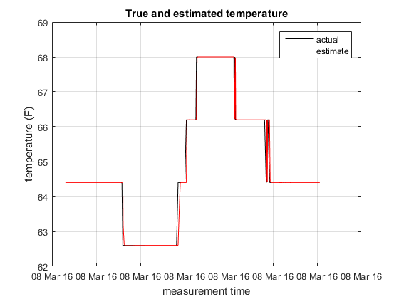The graph above shows the temperature sensor measurement and the estimate. The estimate is following the measure closely here.

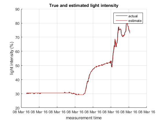
The graph above shows the light sensor measurement and the estimate. The estimate is following the measure closely here.

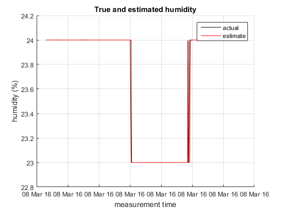The graph above shows the humidity sensor measurement and the estimate. The estimate is following the measure closely here.

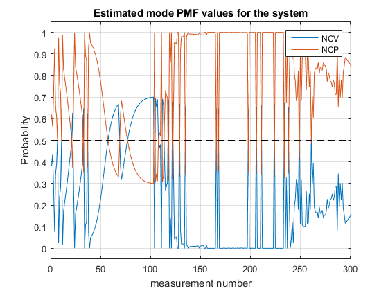The graph above shows the probability the system is in a given mode. You can see this graph working when the system is not changing it tends to be in NCP mode and when the system does start to change it is in NCV mode more. One aspect of coupling these sensors is that the mode needs to account for all 3 sensor changes at the same time. You can see this occurring with this graph.

Data set 2: noisy humidity sensor (set 1)

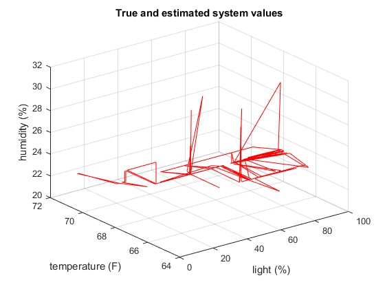
Above is the entire system plotted on a 3D graph to give an idea of the big picture of what is being estimated. This is clearly a more noisy system.

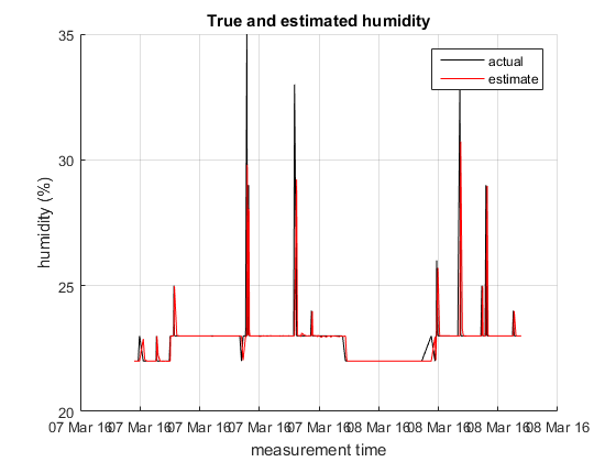
The graph above shows the humidity sensor measurement and the estimate. The filter does not believe this noisy data as much so the actual and the estimates are different. In this case the estimate of the humidity is more accurate than the actual measurement.

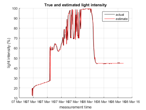The graph above shows the light sensor measurement and the estimate. This measurement is also more noisy. The filter still follows the data pretty well.

The graph above shows the temperature sensor measurement and the estimate. The estimate is following the measure closely here.

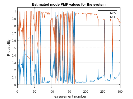The graph above shows the probability the system is in a given mode. You can see this graph working when the system is not changing it tends to be in NCP mode and when the system does start to change it is in NCV mode more. One aspect of coupling these sensors is that the mode needs to account for all 3 sensor changes at the same time. In the more noisy system the modes are likely to change more. There is also less overall certianty of the actual mode.

Wrap up

I've uploaded the files for this simulation to the site. I'll put the IMM-KF engine in C in the mBed repository for the STM32. This code won't be ready until late July as I'm still working out some of the embedded infrastructure for this entire design. So there will be a part 4: implementation but this won't be until later in the year.