 nh8157
Abstract
It has been more than one month since our last hackaday update. The Kalman filter and the PID were the obstacles that stopped us, which our team had very little knowledge of. In general, we took a step forward with the grid system we proposed and implemented task assignment, auto-routing, collision avoidance, as well as error correction with PID on the system. To make the framework more comprehensive, we also implemented a simulation platform featuring all functions implemented on the real robot. The following post will discuss updates discussed above respectively.
Task Assignment
We found that the original framework we developed (please refer to log ) was naive and not efficient. It would be better if robots can sort out their target destinations before they are on the move. With suggestions from various professors, we began digging into academia, trying to find existing algorithms to tackle the problem. It didn’t take us long to find that the task assignment among multiple robots is similar to the Multiple Travelling Salesman Problem, which is a variation of the (Single) Travelling Salesman Problem and is NP-hard. Most of the optimal algorithms are beyond our scope of understanding. Then we began looking for algorithms that produce suboptimal results and are easier to implement. The one algorithm that we implemented was the decentralized cooperative auction based on random bid generators. I will briefly explain this algorithm below.
At the very beginning, each robot would receive an array of destinations to go to and would calculate the closest destination relative to their current positions. There is a synchronized random number generator among all robots. Before every round of the bidding, all robots would run this number generator, which outputs none-overlapping numbers between 1 and the total number of robots in the system for each robot. Having generated the number, robots would bid in turn based on the random number they got. When it is one robot’s turn to bid, it would broadcast its bid and its cost among all robots. Robots haven’t yet made the bid needed to process the bid made by other robots. If this bid coincides with its own pending bid, it needs to delete this current bid and reselect the next closest, available destination. The robots need to do this auction for m times, each time one robot would have a different random ID (thus would make bids at different orders). In the end, robots would unanimously pick the round of bidding with the least total distance.
Suppose the size of the task is n, the robots are programmed to do m rounds of auction to find the smallest total distance, the time complexity to produce a suboptimal assignment is only O(mn). This is a much lower complexity than the optimal algorithm that needs factorial time.
Due to the time constraint, we could only implement a simplified version of the algorithm, where the auction would only last for one round.

Auto-routing
In a grid system, routing from point A to point B (not considering collision) is easy. We defined the length of each cell in our grid as 30cm; the origin is at the top left corner of the grid, the x coordinate increases as going to the right of the grid, while the y coordinate increases as going to the bottom of the grid. Please refer to figure x for further details of our grid setup. To get from point A to point B, the robot only needs to calculate the differences in x coordinates and y coordinates. The intermediate waypoint would have the same x coordinate as the starting point and the same y coordinate as the destination point.
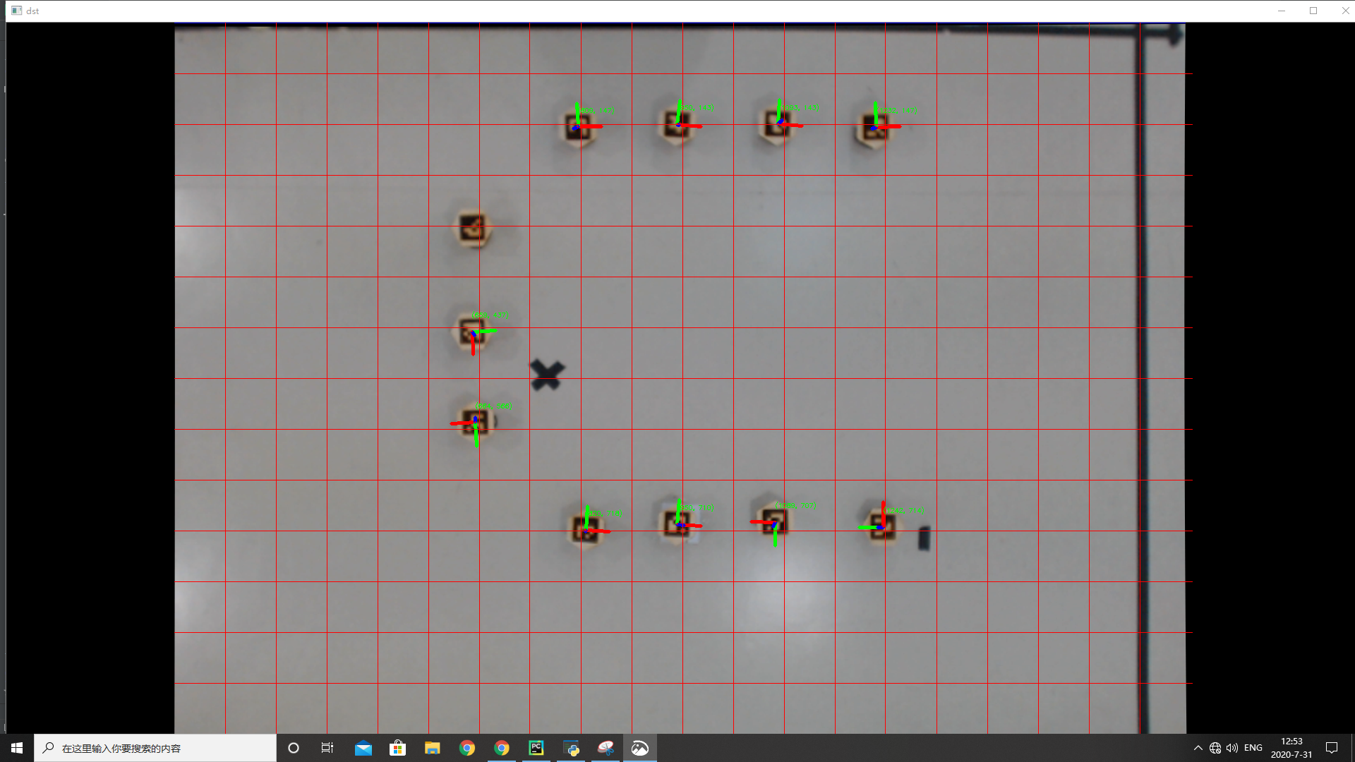
Figure 2. Grid setup
Yet this brute-force way of routing may lead to collisions at various intersections. In a grid system, collisions occur because more than one robot is about to occupy the same coordinate at the same time. Thus, we assumed collisions could be avoided by dispersing the routes of all robots and making them occupy different coordinates at the same time. In academia, there exists many centralized and decentralized solutions for planning collision-free routes. But due to time constraints, the routing we implemented was just a variation of the brute-force way mentioned above. To sufficiently disperse robots’ routes, we exploited the property of the grid system. Suppose a robot needs to get from point A to point B, and the differences in x coordinates and y coordinates are m and n respectively. There would be in total ((m + n) * (m + n - 1) * … * n / n!) many different routes. Based on this knowledge, our auto-routing function generates four waypoints instead of three. The two middle waypoints have random x coordinate values between starting and finishing points.
Collision Avoidance
Despite our effort to implement the collision-free routing function, in practice we still observed frequent collisions among robots. A collision avoidance system based on infrared thus became necessary. Based on other researches, we classified possible collision scenarios in our system as head-to-head collision and intersection collision. Both these two cases have subcases, which are discussed in the figure below.

Figure 3. Classification of collisions
As described in the hardware part above, the infrared receivers and emitters are arranged in a certain pattern. Such a pattern allows robots to detect infrared signals coming from front, left and right. Robots would send infrared signals in a pulsatile manner, where the emitter would be on for 1ms and off for 20ms. Robots use 12-bit analogread to read infrared signals from receivers. The reading ranges from 0 to 4095. The reading has a threshold value, once a reading gets above the threshold, the robot would consider a possible collision from the direction of the receiver that has this reading and output a one.
Based on the readings from the six receivers, we drafted a simple protocol to avoid the collision scenarios mentioned above. Rules are as follow:
1. If a robot receives infrared signal at the front (receiver 3), it would reroute and turn left to avoid the collision from the front.
2. If a robot receives infrared signal at the left (receiver 1 and 2), it would not act.
3. If a robot receives infrared signal at the right (receiver 4 and 5), it would start a random timer. Once the timer expires and no message was received, it would broadcast a message including its ID, current direction, current coordinates.
The order of priority of the collision scenarios is the same as the order above, where the head-to-head collision has the highest priority, then the intersection collision. Inspired by the real-world traffic rules, we determined that at an intersection, the other vehicle coming from the right relative to self has higher priority. In our case, in order to avoid two robots sending out messages simultaneously at an intersection, the vehicle relatively coming from the left would initiate the communication.
Once other robots in the system have received the collision message from case 3, they would compare this coordinate with its current route and try to calculate the collision coordinates between self and other, where the routes of two robots would intersect. If the collision coordinate is both on self and the other robot’s route, this robot would calculate their distances to the collision coordinates respectively. If self is closer to the coordinates, the program would output action 0 for self and action 1 for other, where self would carry on with its task and the other robot needs to stop and wait, vice versa. The action for the other robot, together with the other robot’s ID and the collision coordinate would be broadcast to the rest of the swarm. The initiator would act according to the action given by its peer. For the robot that needs to move along the current route, once it has gone past the collision coordinate, it would broadcast another message indicating it has passed the collision coordinates, so that its peer that stopped could start moving again. The process is similar to computer networking protocol that consists of SYN, SYN/ACK, ACK.

Figure 4. Flow chart for initiator

Figure 5. Flow chart for receiver
Error Correction
It’s important to keep robots running on the grid we constructed. If robots go off-course frequently, the auto-routing functions we wrote would be wasteful, and there would be more possible collision scenarios than we classified earlier. This would drastically complicate the collision avoidance scenarios. There are two reasons behind robots going off-course, first is when robots’ directions are not aligned with north, south, west or east after it turned, second is when robots are going forward, two wheels are not turning at the exact same speed.
PID is one solution to both of the problems. We implemented two PID systems on our robot, one for turning and one for going straight. We only used Kp in both PID systems. In the PID for turning, turning speed is proportional to error. Robot acquires the error locally through the difference between the current encoder ticks and the target encoder ticks (target encoder ticks represent the number of encoder ticks needed to turn a certain angle).
speed = kp * error
Another PID is for bringing an off-course robot back to its course. The robot calculates the error by comparing the absolute coordinate it receives from the camera with the current trajectory it is on. Error is positive if the robot is off-course relative to the right, negative if the robot is off-course relative to the left. This error would be sent into another PID function, which would output two different speeds that the program needs to apply to two wheels, in order to bring the robot back on course.
In practice, we found that having 100% trust in either local information (encoder ticks) or global information (absolute position update) would be faulty. For encoders ticks, though interrupt would update encoder ticks almost instantaneously, the data might be very noisy; for absolute position update, it updates at a much lower frequency (once every second), and there would be certain error between the actual position of the robot and the position advertised by the server (since it takes hundreds of milliseconds for the camera to capture the image, analyze the image and send the coordinates into the LAN). To obtain a cleaner, more accurate error value for PID, we need to implement Kalman filters that do the following:
1. Sensor fusion, which fuses the data from encoder ticks, absolute position update, even IMU.
2. Absolute position error corrector, which would calculate the up-to-date absolute position of the robot based on the delayed position update from the camera, as well as current pose estimation.
Yet it was never easy to implement any Kalman filter. The biggest obstacle was understanding the Kalman filter. We don’t have anyone in our team that is familiar with the Kalman filter, so we have to learn it from ground up. This would not be an easy task. The deeper we dug into this field, the more we felt this would be a mission impossible within 1 month. If we were to devote all our energy to implementing the Kalman filter, the research target would drift from researching multi-agent robotic systems to learning inertial navigation. The latter is already a well-established subject and it would be dangerous if we spend too much time on it.
To solve some of the problems above without any Kalman filter, we implemented timers. After the robot turns for a certain degree, it needs to stop and wait for 1 second before decoding the positional data from the server, which guarantees it getting stable and clean data. If the coordinates received from the server have huge errors compared with the local coordinates, the robot would ignore the current update and wait for the next round of update. If the update still has huge errors, the robot needs to believe in it. We couldn’t solve the delay in the global update, so the robot would rely more on their local encoder ticks instead of the global update.

Figure 6. Flow chart of PID
Production of demo
With all functions above implemented, the system is capable of the following task: user inputs desired destinations’ coordinates, server broadcasts these coordinates among robots, robots then self-assign tasks, plan out a path to reach their own target, finally move towards the target while avoiding collisions. The best demo that can be made out of the current task is shape formation. Inspired by the researchers at Northwestern University, we decided to use our robots to lay out the letters, “N”, “Y”, “U”.
Unfortunately, since the functions/algorithms on our robots are still primitive, we couldn’t lay the robots so densely as Northwestern researchers. Instead, we looked at a 5 * 5 matrix to find out which row, column pairs should be taken up to form each letter. We then mapped this row, column pair to the coordinates in the grid system. When executing theshape formation, we first put the robots on the ground randomly, turned them on, then sent the entire set of coordinates needed for this letter.
We started with letter “Y”, since it only needs 7 robots; then letter “U”; at last letter “N”. The process of preparing the demo was not very smooth. Since the collision avoidance functions were still rather primitive, when we were dealing with letters that need more robots, such as “N”, we encountered numerous deadlocks and edge cases not specified in our program. It would be important that we focus on this field of research in future iterations. Despite the difficulties, we still managed to form the letters as we expected. Please check out the time-lapse video down below.

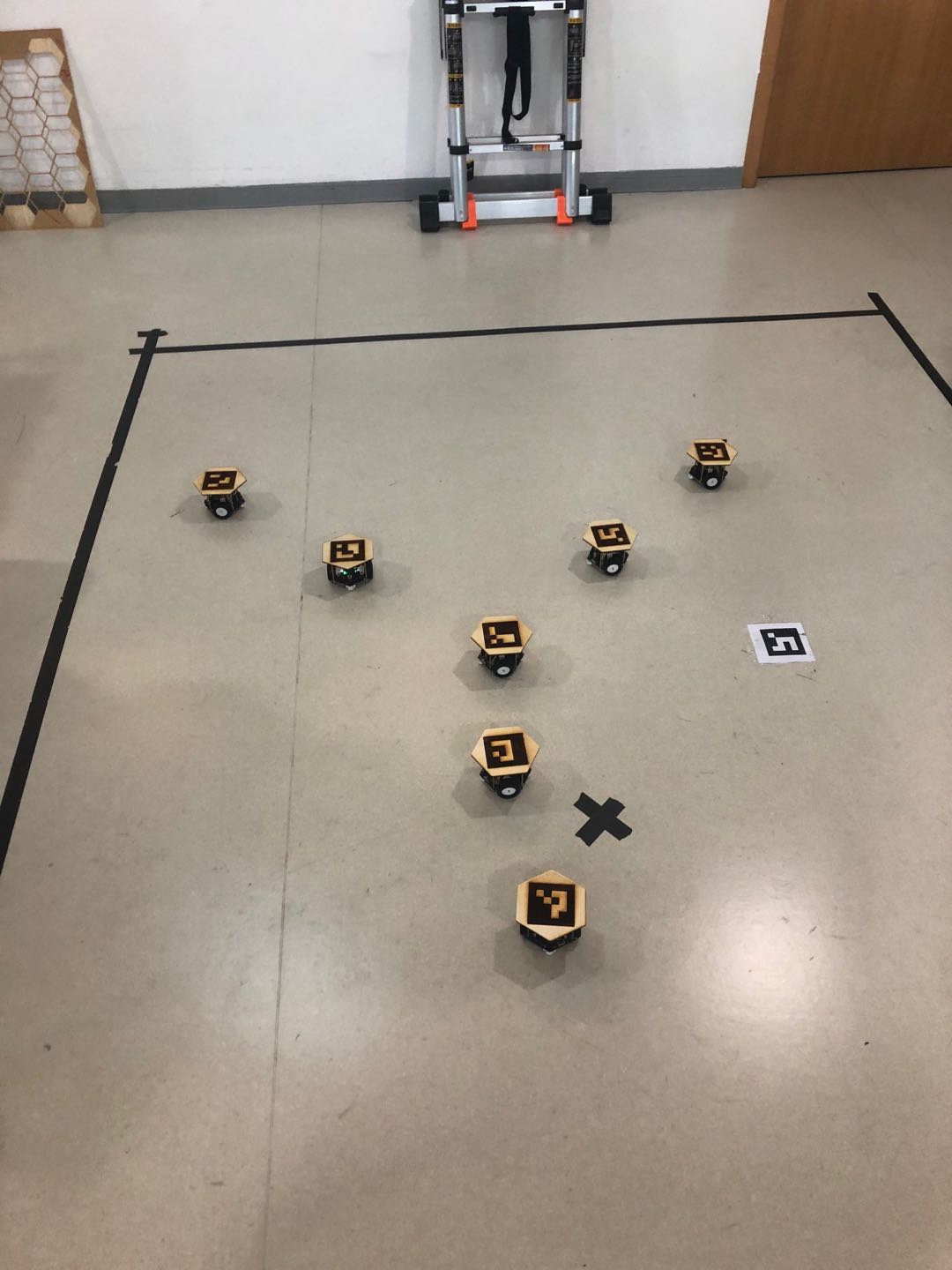

Figure 7. NYU shape formation
Simulation
To better demonstrate our physical field test, we planned to simulate a model that is similar to our real robots in Webots. The first method that came to my mind was that I can simply build a model from scratch using the 3d-modeling functionalities in Webots. As we partly mentioned in the past blog posts, 3d-modeling in Webots is “component-based”. To build a model, we need to create each of its components and assemble them together. In the case of building our robots, we need to create components like wheels, robots’ body parts, various sensors, and etc. (Please refer to Figure 8 for more details). It is interesting to note that if we want to code some functional parts like motors and sensors, we have to use components designated in Webots.

However, considering that our robots are hexagonal, those functionalities could only enable me to create a robot model in some regular shapes like linear, square, and circle, which is not similar to our physical robots. Therefore, we decided to import our 3d-model file of our real robots into Webots to demonstrate a robot model that is really similar to the real ones. This process is pretty tricky. The format of our 3d-model file is .stl while the needed format by Webots is .proto, which is specially used in Webots. Since we had no idea how to convert .stl to .proto, we dug into investigation of the conversion. We could not simply find an existing online platform that enabled us to complete such a conversion. Luckily, we did find a solution that we could convert .stl to .proto with the help of “xacro” language in ROS. Along with the .stl file, we needed to create a new .xacro file, which is used to define the model in .stl file in its shape, mass, core, and etc. After we had those two files needed, we used a python module named “urdf2webots” to convert those two files into a .proto file, which can be imported into Webots.
After we successfully imported our 3d-model, we created other components like motors, wheels, and sensors using the basic nodes in Webots and assembled them together. As mentioned above, using the basic nodes in Webots is to help us better code them, for example, code the motors and wheels to make the robots move. To this stage, our simulation robots seemed pretty similar in shape and size to our real ones. However, the color and texture are distinct because these two features require a lot of texture files to add onto the robot model. Since those files are difficult to obtain and unlike the shape and structure of the robots, such appearance can hardly affect our test result, we chose to ignore the color and texture of our robot model in Webots.
Below are three pictures that can demonstrate our models.


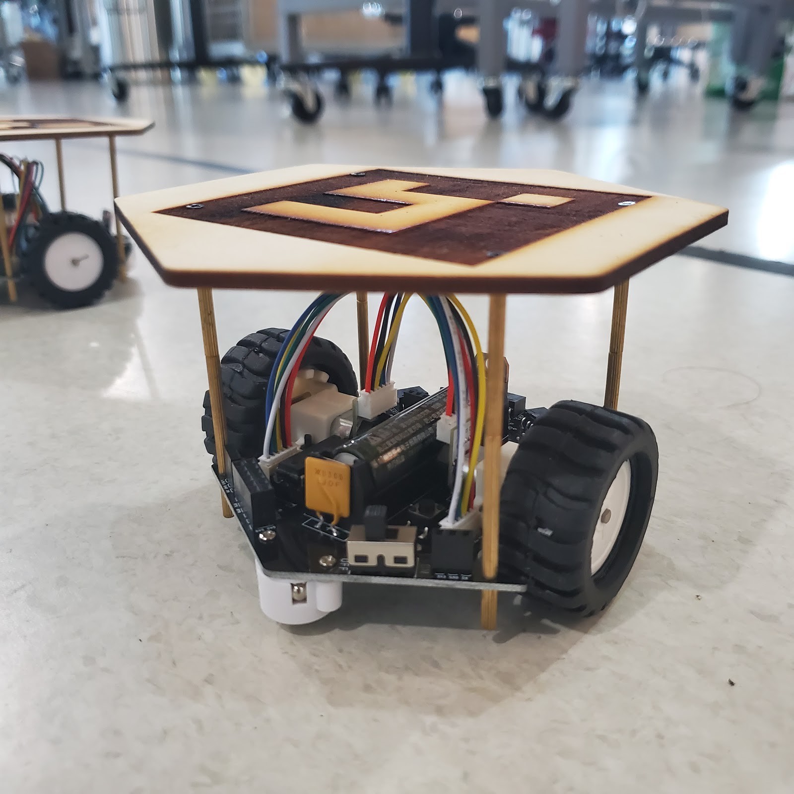
From top to bottom: our first model that was made merely by the basic nodes in Webots; our current model that is created by combining basic nodes in Webots and our imported 3d-model together; our real robot model.
We adapted our real code onto Webots robot controller after we finished building our robot model. As we mentioned above, we have functions including task assignment, auto routing, collision avoidance, and error correction. By simulating and running many tests on Webots, we found out that both task assignment and auto routing work very well on Webots, which is very similar to our physical test. All the robots are able to process the data given by the server and decide its path to its desired destination. (Below is a picture to display the result of one test. This test is to let the robots form a pentagon, where the robots will receive the five points of the pentagon and decide where to go).

Figure 9. Robots form a pentagon
As for the error correction part, we still need to implement PID in the simulation even if we do not have to worry about the technical defects of the robots’ components in real life. In other words, robots in simulation will also go off-course either when moving straight or turning, but just for a different reason. The reason is that in Webots we can not program robots to specify a movement, either forward or turn, in a certain amount of distance or degree. Since we only know the speed of its forwarding or turning, we chose to use time to control the distance and degree. However, this method will cause small errors each time the robots conduct a movement because the rotational motors of the robots can never stop right on time, so they will rotate either more or less than expected. The implementation of PID control greatly reduced the cumulative caused by such small errors. It helps us minimize the error to about 3 millimeters in both x-axis and y-axis. Considering the size of our robots which is around 10 centimeters in length, 10 centimeters in width, and 8 centimeters in height, such an error is very small.
As for the error correction part, we still need to implement PID in the simulation even if we do not have to worry about the technical defects of the robots’ components in real life. In other words, robots in simulation will also go off-course either when moving straight or turning, but just for a different reason. The reason is that in Webots we can not program robots to specify a movement, either forward or turn, in a certain amount of distance or degree. Since we only know the speed of its forwarding or turning, we chose to use time to control the distance and degree. However, this method will cause small errors each time the robots conduct a movement because the rotational motors of the robots can never stop right on time, so they will rotate either more or less than expected. The implementation of PID control greatly reduces the cumulative caused by such small errors. It helps us minimize the error to about 3 millimeters in both x-axis and y-axis. Considering the size of our robots which is around 10 centimeters in length, 10 centimeters in width, and 8 centimeters in height, such an error is very small.

Figure 10. Distance sensors in Webots
Another major obstacle is that the distance sensors in Webots can only detect “Solid”, which is a property of the components in Webots. Generally speaking, many of the basic nodes in Webots have such Solid property, like the motors, wheels, sensors, and etc. In other words, they can be detected by the distance sensor. However, since the body part of our current robot model is imported and is not a basic node, it doesn’t have the Solid property, so it can not be detected by the distance sensor (we did research in the API Functions of Webots to come up with this conclusion). To cope with this issue, we manually added four “borders” onto the robots using the basic node in Webots called “Shape”, which is displayed in yellow in the Figure X + 7 below. We adjust its length, width, and height to enable distance sensors to detect it better.

Figure 11. Four borders
Discussions
Become a Hackaday.io Member
Create an account to leave a comment. Already have an account? Log In.