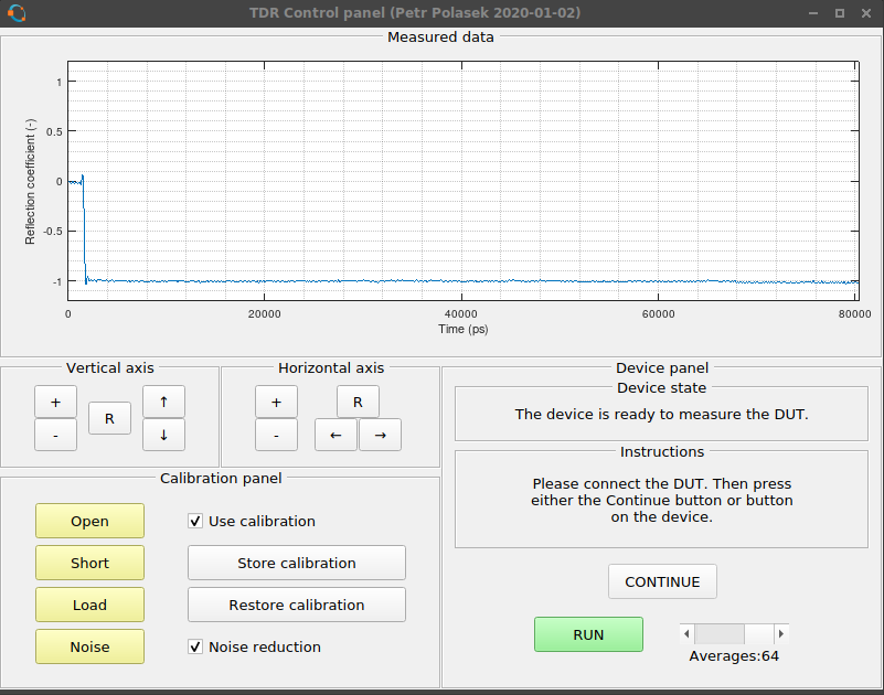
 MS-BOSS
Last time, I mentioned I was having some problems with the open-short-load calibration. I didn't know what was going on, supervisor of my diploma thesis had no clues as well and even none of my friends could help me. This time I will tell you the result of this log in the first article: I fixed it.
What was going wrong
When I performed the calibration, it seemed to be somewhat unstable. To make this statement less euphemistic, it was unusable, totally. After the calibration, I checked that applying the calibration onto the data used when performing the calibration, the result was correct. At t=0, there was the correct reflection coefficient and everywhere else were zeros.
However, after measuring the same calibration standard again (and even without disconnecting it and then reconnecting), the results were off. The peak reflection coefficient was slightly off from t=0, didn't reach 1 or -1 and was not a single-point peak. It was dispersed over several points.
Expectation can be the biggest mistake
I thought this was completely bad. However, it turned out that calibration cannot guarantee that the results will be perfect. It may look so in spectrum domain, but the end result in time domain can be quite unexpected. It was mostly my fault, because I was expecting too good results. And it looked really bad, because when the TDR response is shown as impulse response instead of step response, it looks different and not that intuitive.
So, I started with integrating the result after calibration. A simple algorithm which makes each point a sum of itself with the preceding point and iterating from t=0 to the end of the dataset did the job. However, the results were horrible. After re-measuring the calibration standards, everything looked quite normal.
But after connecting a cable between the calibration point (end of first cable) and the calibration standard, the result was covered in some periodic noise. And it was large!
Really, that makes no sense. Both I and my supervisor didn't know what was going on. I tried recreating the equations for calibration from 4 different articles/books only to come up with the same set equations in the end. I even checked them with wxMaxima (great tool, if you need something like Maple, go and get it), all looked OK. But the calibration didn't work. I thought there could be a problem with the FFT/IFFT but couldn't find out what it was. I thought it could be the DC part of the signal or the fact that the measured signal isn't periodic. So I thought I could use windowing in the FFT to mitigate this possible problem. However, when you look into the equations of the calibration, the windowing would disappear in the end (except for points where the window equals 0). So no luck using that. And so I thought it was just damned and that I'm an idiot.
Yesterday, I thought whether differentiating the measured dataset could help. Simply said, each point in the dataset after differentation equals its original value minus value of the previous point. And... it worked.
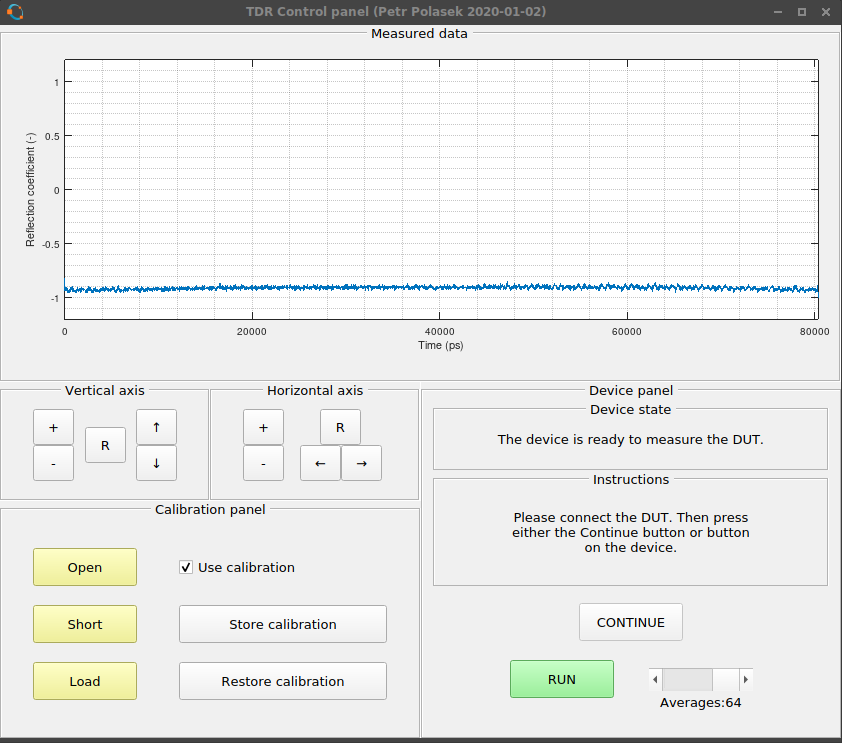
So, from this:
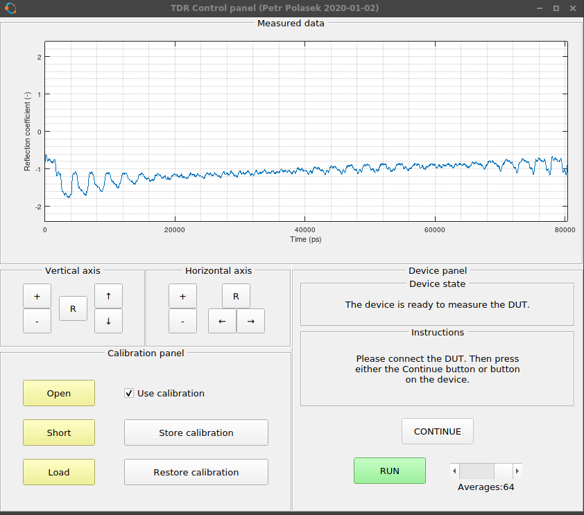
I got this:
It was not perfect, but substantially better. The "blip" on 16 ns caused by reflection on the connector of the reflectometer was gone. Overshoot and ringing on the edge? Gone. Noise? A lot of it emerged from nowhere.
So, the calibration started to work. However, there was a LOT of noise. Way too much noise.
When you feel like there is too much noise, get yourself a wiener
Sorry, it should be Wiener with large W. But I couldn't resist playing with the word. The proper term is Wiener deconvolution. In this case, it is a bit simplified. The deconvolution uses an estimation of spectrum of the original signal and spectrum of noise of the piece of equipment.
So, how it works? I expanded the calibration by one more standard called simply "Noise". First, you have to measure the "Load" standard on maximum averaging and saving it, then measuring the same standard without averaging and saving it as "noise". The software then subtracts these to get only noise. Then it is properly scaled according to the number of averages used when obtaining the "load" and "noise" standards. And the number of averages used when performing new measurement. To remind you, the noise lowers with 1/sqrt(N) where N is the number of averages. I thought it was 1/N and had a half-working code for several hours. The "load" standard is used as a reference of noise in the Wiener deconvolution and the "noise" ... as noise.
So, when the data is to be shown, you can check a new checkbox to enable the noise reduction. It doesn't matter if you run it on the calibrated or uncalibrated data, it works the same. And it works quite good.
Now the noise is heavily suppressed. Not completely, but it is acceptable now. Trying to get less noise also causes the waveform to be too smooth. The edges then get slower and slower, some small details are completely smoothed out and ringing reappers.
So, how does the damn Wiener work? The equation for the filter is

Multiply the spectrum of the measured data with this filter. The parts of spectrum where the signal reaches noise floor get heavily attenuated. So, noise is attenuated and clean signal is not. Remember, the SNR is a POWER variable so it depends quadratically on the noise and the reference signal.
This gets us back to the reference signal. What is it? Something that looks like the pulse from the pulse generator. I used probability density function. It is similar to the generated pulse and if you integrate it, the result equals to 1. So, it doesn't rescale the waveform.
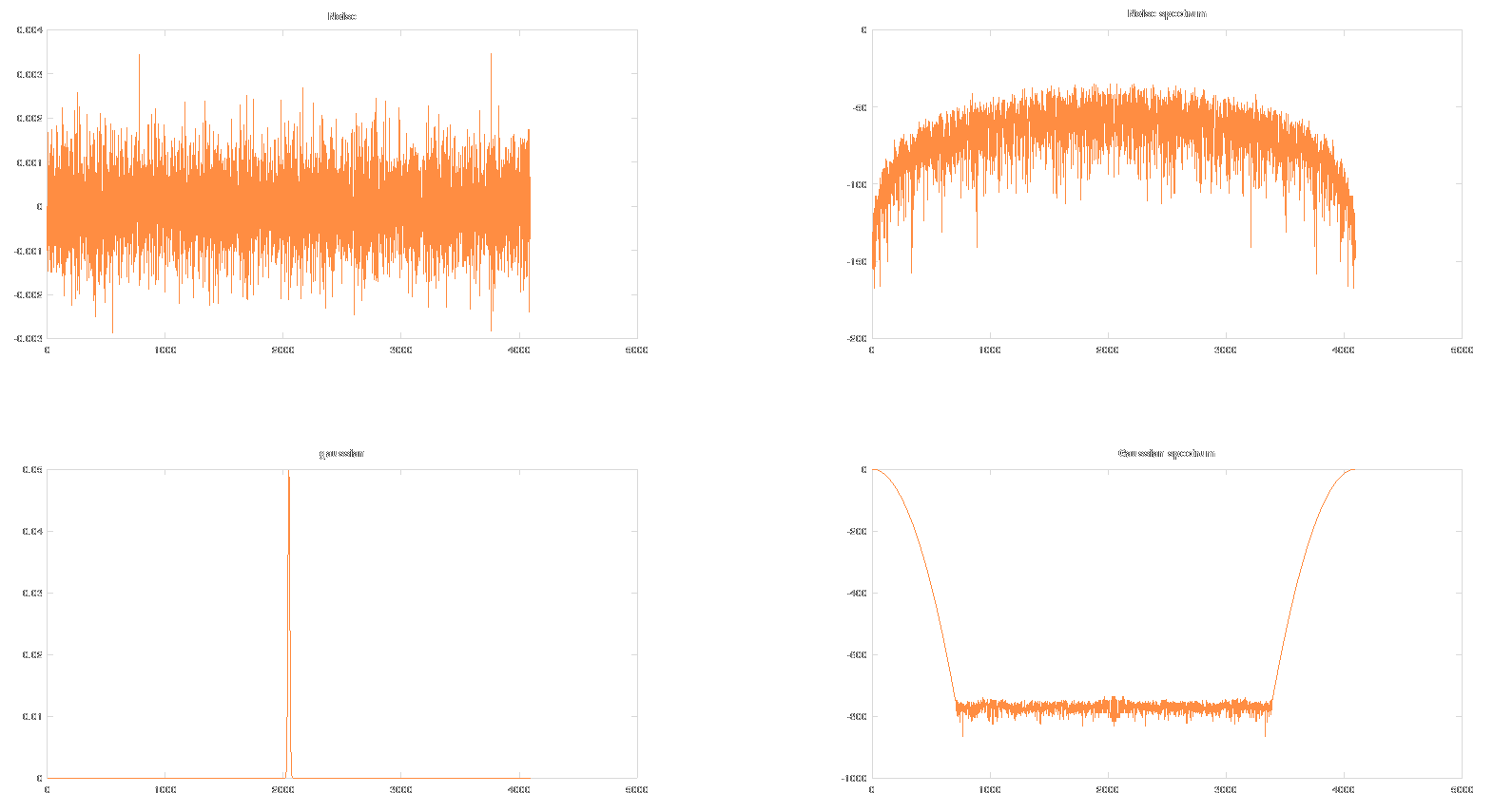
In the graphs above, you can see the measured noise, its spectrum (it is the dual-sided FFT spectrum). Then the gaussian (not very well visible, sorry) and its spectrum.
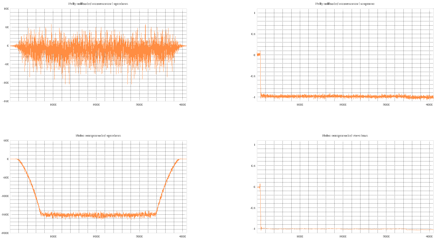
Now, in the graphs above, you can see the original spectrum and waveform of the calibrated waveform. under it, there is the version with reduced noise. As you can see, most of the spectrum is completely suppressed and the rest is bent so that it more closely represents the reference signal instead of noise.
To explain why the missing parts of spectrum aren't missed by me at all is simple. The reflectometer samples at 50 GSa/s. This allows noise up to 25 GHz. However, the bandwidth of the analog frontend is more like 2.5 GHz. This means that out of the 25 GHz bandwidth, 22.5 GHz of it is more or less only noise. And nobody likes noise (except in photos, noise reduction usually only hurts them).
One-port VNA calibration
The one-port calibration is simple for the user. Attach a calibration standard, measure it, save it. And do it for all three standards (and the noise!). Check a checkbox and it's done. However, inside the black box, a lot is going on. But only a small portion of it is the calibration itself.
S11L=fft([0 diff(calibration_data.load)]);
S11O=fft([0 diff(calibration_data.open)]);
S11S=fft([0 diff(calibration_data.short)]);
S11M=fft([0 diff(decoded_data)]);

Ed=S11L;
Er=2.*( ( (S11O-S11L).*(S11S - S11L) ) ./ (S11S-S11O) );
Es=-( (S11S+S11O-2.*S11L) ./ (S11S-S11O) );

S11A= (S11M-Ed) ./ ( Es.*(S11M-Ed)+Er );
As you can see, it takes the three standards, differentiates the and then gets their spectra. The same happens for the measured dataset. Then it calculates three error properties of a two-port error network. Three unknown vectors computed from three vectors. Then, it applies these three error properties onto the measured vector. And that's all.
Maybe you remember that a two-port network should be described by four parameters. However, since we are using only one port and can measure only in one way, we are only interested by going "through" the network only in one way. So, one of the variables is fixed to value 1 and made part of one of the three remaining parameters.
The result is that the DC offset, scaling error, reflections from the connector and cable and multiple reflections are suppressed. And the waveform also get sharpened. As much, as it can be sharpened. And that is why a lot of noise emerges. Sharpening amplifies high frequencies.
However, I will not give a complete lecture on VNA calibration since I am not an expert in this area.
See you soon in another log or project!
Discussions
Become a Hackaday.io Member
Create an account to leave a comment. Already have an account? Log In.