 Charlie Smith
In the previous log I finally managed to get IQ data, and with that the next set of problems. Firstly it seems that my data is very noisy and while I have made some improvements on that front, for this log I want to talk a bit more about simulations. I also promised to talk about running the MUSIC algorithm in real time on the nRF52833. However, that will also be in a later log, probably when I have direction finding working (so hopefully the next one but who knows).
Firstly I would like to note that at the end of the previous log I suggested that one of the issues is that because the IQ data should have a frequency of 250kHz, then I should have been using this frequency in the MUSIC algorithm. This is wrong. At some point I found this page which eventual (look for a post near the end by robwasab) points out that a phase shift in the 250kHz baseband frequency will be equivalent to a phase shift at the 2.4GHz radio frequency. Thus, while the IQ data propagates at the lower frequency, the initial phase shift seen between sets of samples from each antenna is still based on the higher frequency. I think this is poorly explained by the documentation but it at least means we may not need a much larger array size to get AoA data. This also made me think about the what might be the best radius. I was initially thinking that I should probably have a larger radius anyway, but as we shall soon see from simulations, I may need to do the opposite and make the radius smaller.
Simulated Signals
For running simulations I am using a Python implementation of MUSIC. This not only performs the actual calculations, but also generates the simulated data from each antenna. This simulated signal is crucial to being able to make useful predictions from the simulations. If it is done wrong or poorly then I might as well not bother with simulations at all.
To get a fairly accurate phase value we can consider a spherical wave from a source point R, traveling to each antenna at positions r_i. Then we can found the number of times the wave will cycle over the distance to get w_c. This will be some integer multiple of the wavelength plus an additional fraction to get a relative phase ψ_i. This phase isn't really relative to anything in particular, but can be made so by subtracting the phase from some reference point. As the phase of the data we measure is fairly arbitrary anyway this can probably be ignored.
Using this, we can then add some amount of Gaussian white noise and we get a sample. To match what we can measure we can then make a number of samples by progressively offsetting the phase by 2π*250000*dt. Where dt is the time step between samples. I should note that each sample should have its own noise, rather than applying the same noise to all samples for each antenna. This should give a fairly accurate simulated signal base on the position of the source which we can vary over time. The only issue being that the noise being added is probably not really the noise that we actually see, but it will do for now.
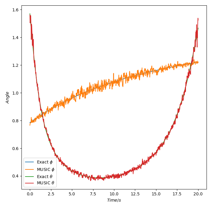
We can also consider some examples for the typical motion we might see The first of these is some simple projectile motion based on an initial velocity and position. This is roughly what you might expect from throwing the beacon, or putting it on a model rocket (which was sort of the original aim of this project). This is the motion I have used for the simulated data shown previously. For the graph shown we use a radius of 45mm and a 1% phase error.
 Now let us consider a second test case. This is a bit more random, but is going to be sort of equivalent to running in circles around the receiver and waving the beacon around in the air.
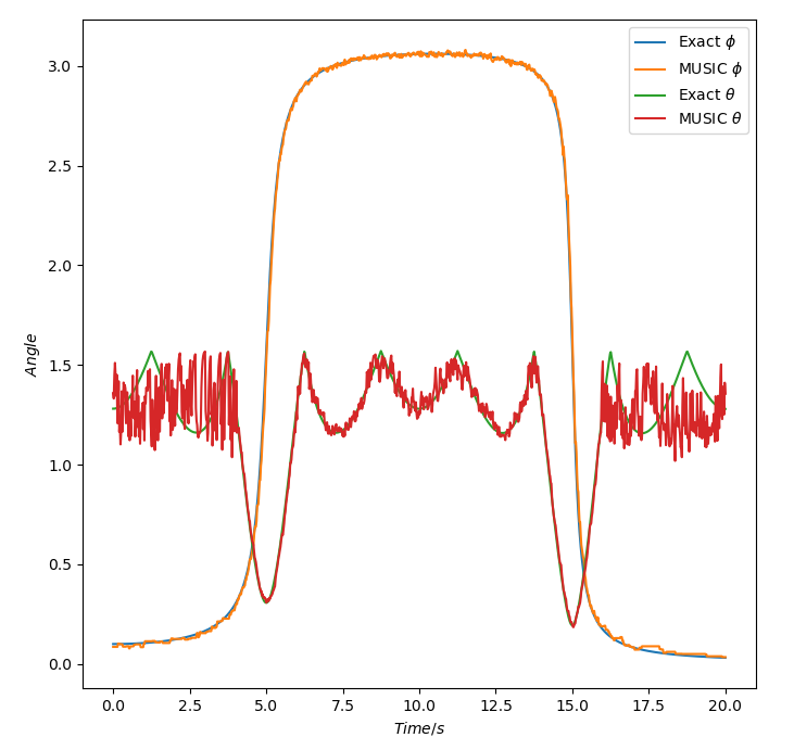 Doesn't look too bad, but the start and end good do with some improvement. Well we where thinking of using a larger radius, so lets look at using r=100mm:
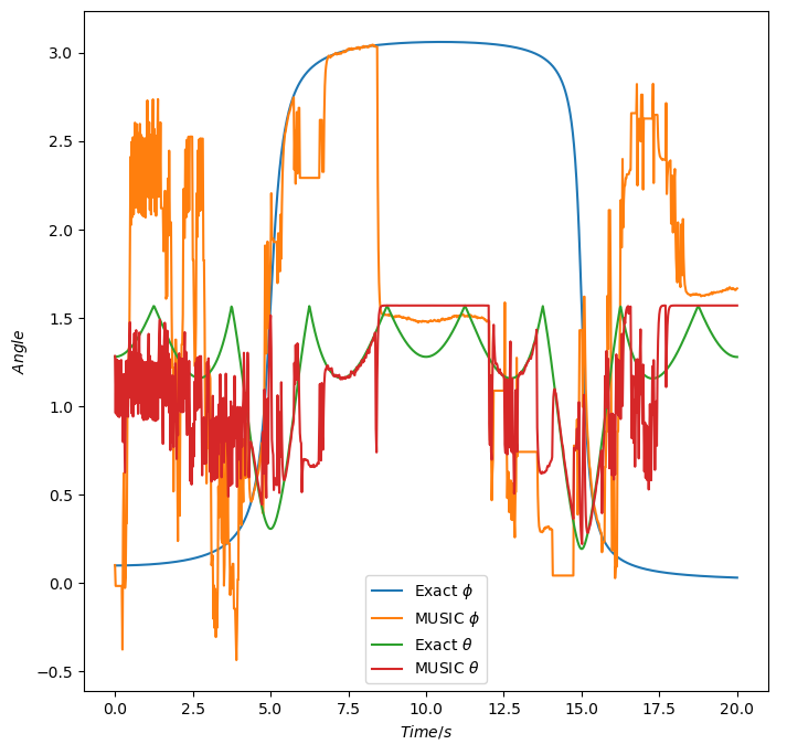 Oh. Well that's quite a bit worse. So why could this have happened, is there some upper limit to the radius we can use? Well yes actually there is, due to the MUSIC algorithm. In this paper it states that we when the spacing between antennas for a uniform linear array is greater than half the wavelength then we will see multiple peaks in the MUSIC spectrum and so no longer be able to tell what the angle is. This is possibly the problem. However we are using a circular array, not a linear one, so how does this apply here. If we consider the circle as just a curved linear array that joins end to end, then the antennas spacing we should consider is the distance between antennas along the circumference giving us the limit on the radius of:
Changing The Radius
Rather than going though and manually generating the graph for a number of values of r, it is much better to run lots of simulations and directly generate a graph for quite a range of values. To get a good idea of the full range of possible values, lets start at a 5mm radius and go all the way to a 500mm radius. As a note, these also still have a low pass filter over the AoA data.
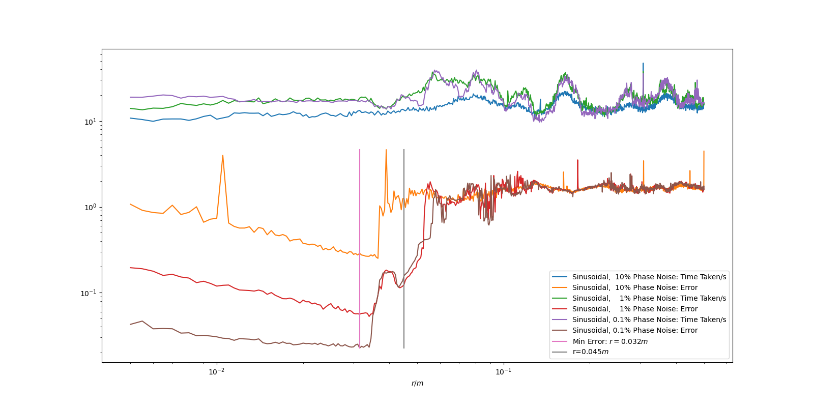
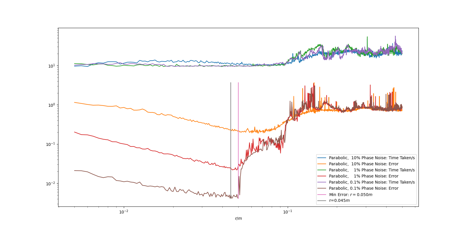
This data is quite noisy, but it very clearly shows what we sort of expected. The data gets better as the radius increased, but at a certain point it then gets worse again. Having a lower noise also gives a lower error, but also seems to limit the maximum radius before the increase in error. Interestingly above about r=100mm, the error is independent of the noise in the measurement, clearly due to this error being from the algorithm no longer being valid. This behaviour is present in both the parabolic and sinusoidal test case. However in the slower moving parabolic motion, the radius can be quite a bit higher. This is likely due to the low pass filter being used on the data.
What we really want is the worse case scenario as a test case to find the maximum radius, but clearly I can't test every possible motion. However we can at least see that the radius of 45mm currently being used is often above the maximum. I also hypothesise that the the diameter of the array must not exceed half the wavelength. For 2.4GHz this gives a maximum radius of 31mm, which is below an limit we have seen in the test cases used. However this has not been tested at other frequencies and so may just be a coincidence. It is also not tested on actual hardware, but hopefully I can do that at some point in the future.
That will do for this log. I thought this was quite an interesting way to further investigate the properties of my system through simulation. Of course it is only a simulation and so may not apply directly, but it is still a useful tool, and I think it should be used when possible. I have also made some progress with the hardware side, notably finding that I was not using the correct control signals when selecting which antenna to use. I also may need to add a -3V3 supply to allow the RF switches to switch between antennas faster, but I still need to look into how exactly I will do that. Finally, my hope to find a low cost VNA have been significantly improved after the nanoVNA V2 was pointed out to me on Twitter. I have not yet ordered one, as it seems a new version should be released in a week or two, which should have lower noise and sweep frequencies faster for the same price.
Thank you for continuing to follow this project, hopefully I have some more exciting updates soon. But in the meantime feel free to leave any questions you have, and I will do my best to answer them in future logs.
Discussions
Become a Hackaday.io Member
Create an account to leave a comment. Already have an account? Log In.