Phil Malone
A search for related projects
I always start out new projects be making sure I don't re-invent the wheel.
A quick check of ongoing Hackaday (and other) projects returned many examples of visual spectrum analyzers. Some of them are simple LED strips, and others are full Matrix displays. Some use a microphone for their input; others use line inputs, Bluetooth or even audio files. Other major variations between different analyzers were the number of specific frequency bands that are measured, and how the signal strengths are displayed.
None of the ones I found had anywhere near enough Bands form my liking, so I decided it was worth continuing with my project.
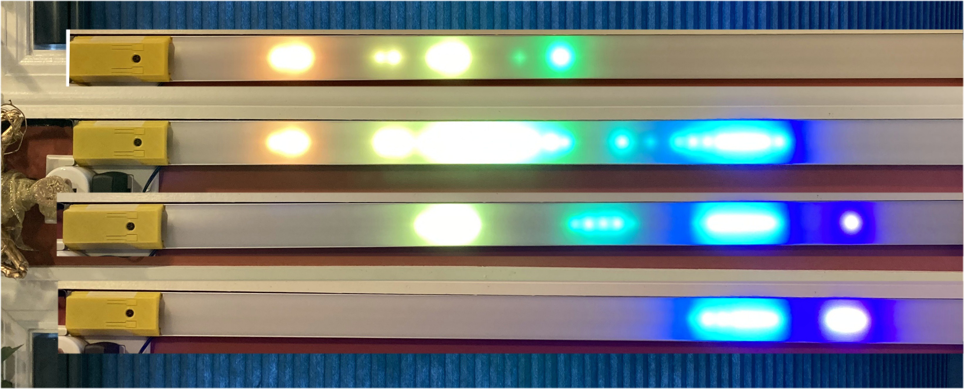
Sometimes it's more fun to show where I'm at now, and then explain how I got there.. So here are my current specs.
- Display Bands: 104 Bands, spanning 43 Hz - 16744 Hz (8.5 Octaves)
- Each Band is displayed with a specific color, and 512 intensity levels (Using 2 LEDS per band)
- Display is updated with fresh data every 11.6 mSec (86 Hz update rate)
- Visual Latency: 13.5 mSec (11.6 mSec acquisition + 1.9 mSec for dual FFT & display)
- Low Freq (<800 Hz) Persistence: 185 mSec.
- High Frequency (> 880 Hz) Persistence: 46 mSec.
This video is for an earlier version with the same number of bands, but a longer latency and slower update rate.
But, going back to the beginning... I find it useful to start my projects with a rough set of system Requirements. This helps me to clarify my goals, and it gives me a place to return to when it's time for me to evaluate how well (or otherwise) the project is going.
So my first Project log will start there, and then we'll see how it goes.
- Log 1. System Requirements
- Log 2. Things I learn along the way
- Log 3. Optimizing performance to meet requirements
- Log 4. A processor Upgrade
- Log 5. Making it look nice
- Log 6. Pushing the performance envelope
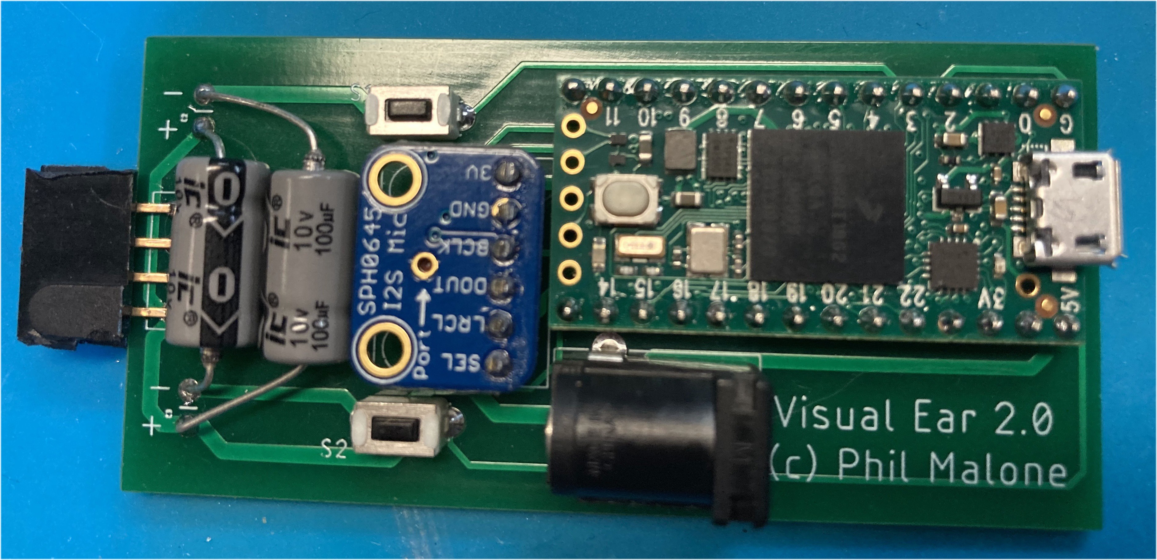
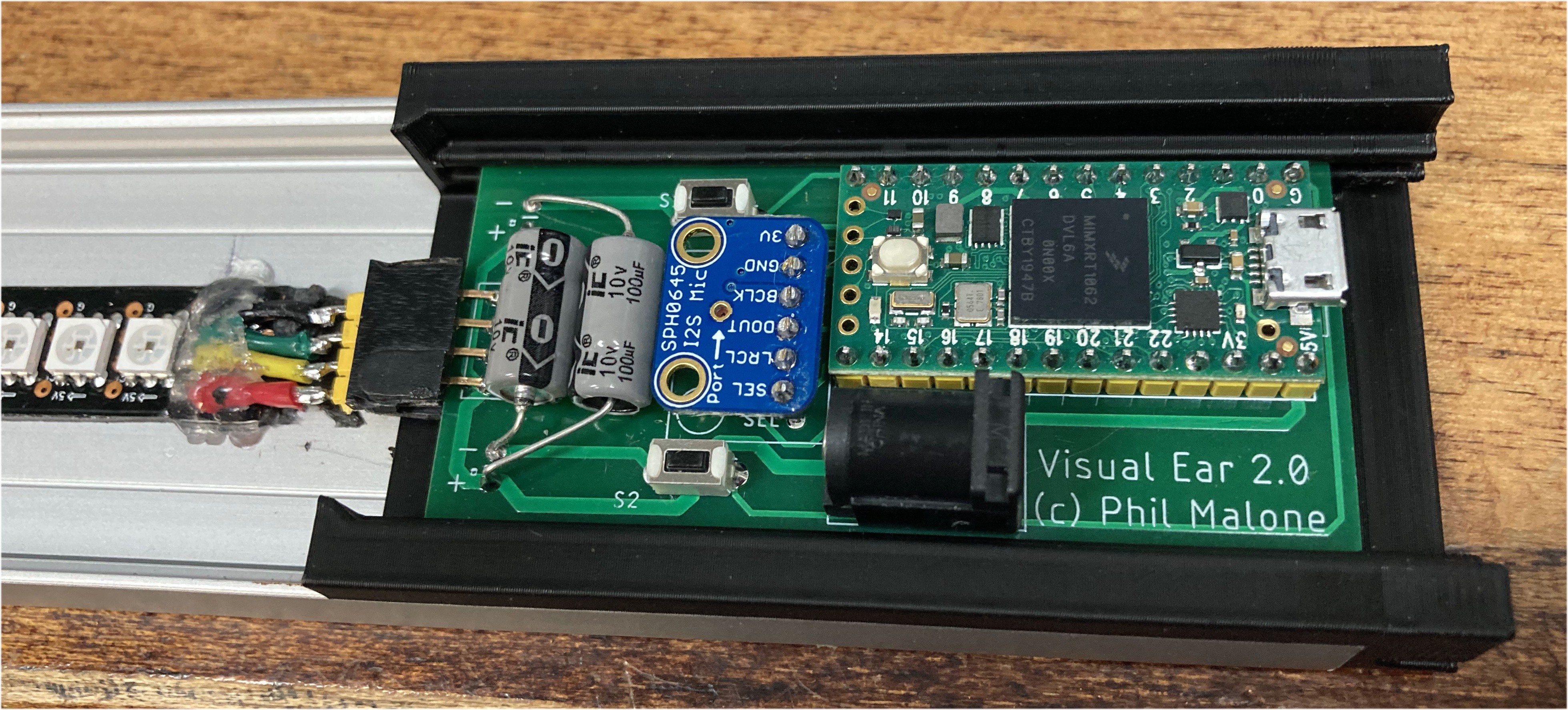
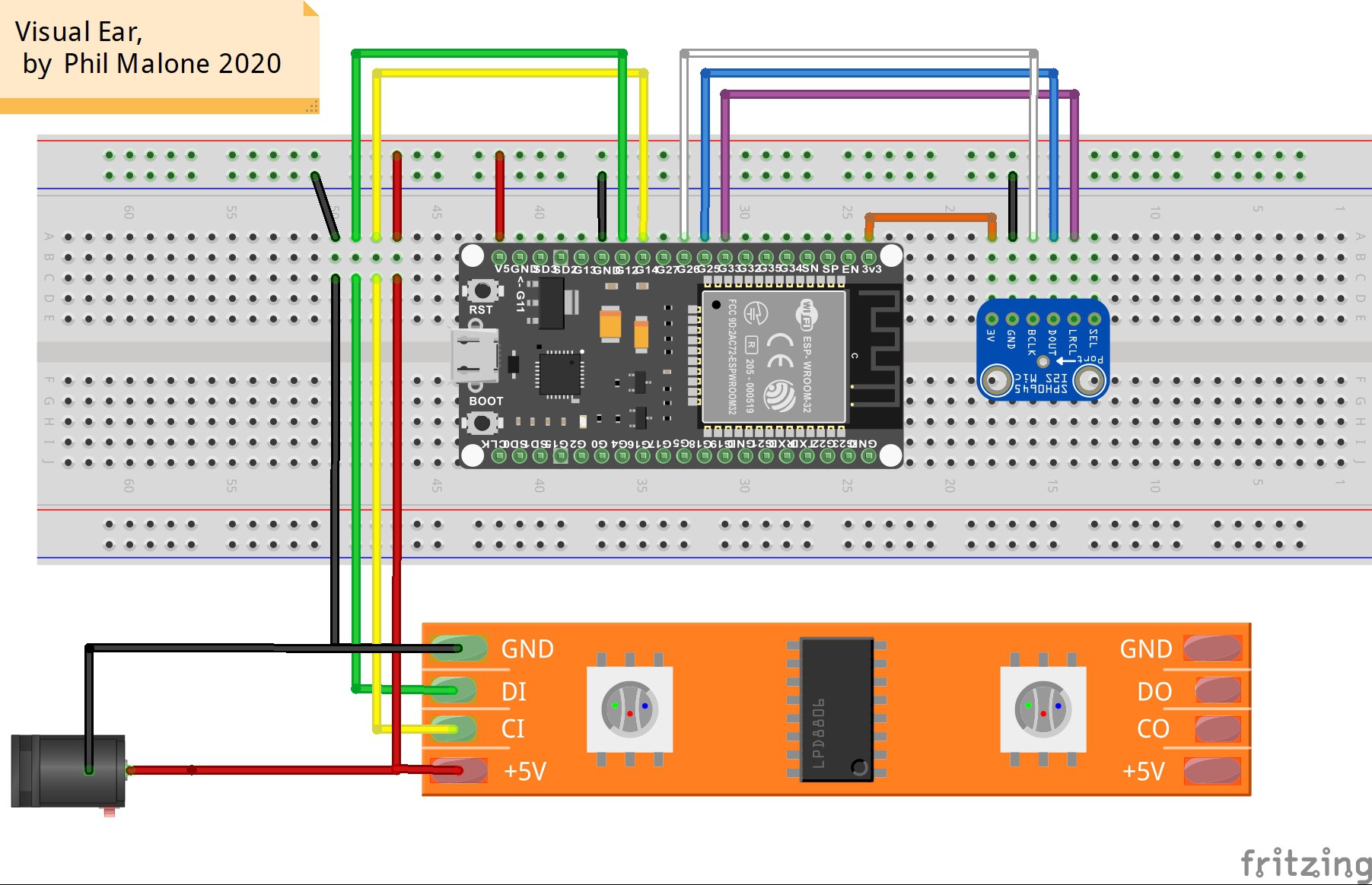
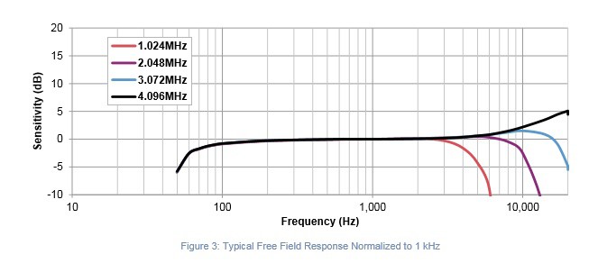 I2S: - SPH0645LM4H
 tshen2