Theory

Passive Sonar

As an alternative to measurement of vehicle motion using a radar gun, I wanted to build a very low cost system which didn't require illumination of the vehicle either actively with a local source (monostatic radar/sonar) or passively (bistatic radar/sonar).  The acoustic energy generated by the vehicle itself can be used to locate the vehicle by measuring the angular direction of the source of the sound.  This is called passive sonar, very similar to the type of sonar performed on submarines to locate other ships, for example.

Doppler Shift

My first approach was to see if I could measure the Doppler shift of the road noise as a vehicle passes by the sensor, just like a siren on an emergency vehicle displays a shift in pitch as it travels past the listener.  I found out that there is no detectable Doppler shift of the road noise because the primary sources of the noise are not on the vehicle itself, but rather arise from the impact of the tires on the rough surface of the road.  Since the noise is coming from the road which is not moving with respect to the listener, there is no Doppler shift.

Time Correlation

The basic idea behind passive sonar is to use two or more microphones to measure the sound emitted by a moving vehicle and determine the difference in time between the signal arrival at the sensors.

There are existing systems which use time of arrival (TOA) to locate the source of sounds using triangulation geometry.  However in my particular application the time of flight is short and the time differences between microphones will be relatively small compared to the wavelength of the sound.  Rather, this measurement will capture the phase difference of a sound wave measured at two closely spaced microphones.  This is similar to phase interferometry used in radio astronomy and presumably used in some other acoustic-based locating systems.

The basic geometry is shown in Figure 1 where D is the distance from the microphone baseline to the roadway, b is the separation between microphones, x is the lateral position of the vehicle from the center of the microphone array, and θ is the angle between the baseline and the direction to the vehicle.  The distance from the left microphone to the vehicle will be different from the distance from the right microphone to the vehicle by the amount δ_t ∙ v_s where δ_t is the time delay of the sound signal between the two microphones and v_s is the speed of sound.

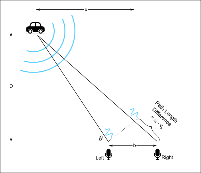
If we assume a plane wave approximation to the sound wave at the microphones, the relationship between the vehicle position, x, and the time delay becomes:

As the vehicle passes the sensor array, the measured time delay will map out a smooth function and, in principle, the vehicle speed can be extracted.

Hardware

A basic constraint for this project is to keep the cost of hardware as low as possible, so I chose to leverage a Raspberry Pi computer since the linux operating system supports stereo audio natively and USB sound cards with stereo microphone inputs are low cost.  Since the speed of sound is about 343 m/s at room temperature and sea level, if the microphones are spaced 1 meter apart the maximum time delay will be about +/- 3 ms.  Typical audio sample rates are 44.1 kHz or 48kHz which should be sufficient to capture a time difference of 3 ms.

One important consideration in performing this measurement is that both microphones be identical in performance.  So the acoustic response should be as close to matched as is practical, as well as the gain and phase response of the electronic signals.  Some digital microphone systems have internal variable gain control and automatic noise-cancelling features which can disrupt a precise phase delay measurement such as this, so to ensure a stable gain and phase response and also minimize hardware cost I chose to build my own microphone and preamp with a fixed hardware gain.

For the microphone construction, I used two Adafruit 1063 electret microphone and preamp boards.  I discovered two limitations of the preamp circuit which needed to be solved.  First is the board requires a very quiet DC power supply since any ripple on the supply is largely unfiltered by the board and fed directly into the preamp input.  Secondly, the board needs to drive a cable to the sound card input port and the stray capacitance on this cable can exceed that allowed by the MAX4466 amplifier to ensure stability.  So a series resistor is required to drive the signal cable.  Since the microphones need to be separated by about 1 meter and the power supply needed to be close to the preamp board, I removed the microphone element from the preamp board and used a single power supply board with both preamp circuits mounted on it.  I also wanted to power the preamps from the USB power supply of the Raspberry Pi computer which is very noisy, so a high performance power converter is needed.  I designed a simple DC-DC converter to take the USB power and generate 7V DC which is then filtered and regulated to a quiet 5V supply for the preamps.  Another very important consideration in constructing any microphone is proper electrical shielding of the condenser and cable.  I constructed an enclosure for the condenser from brass tubing and wire screen and used shielded audio cable to provide a 1 meter length from preamp to condenser.  The screened condenser was then placed inside a PVC pipe lined with open-cell foam to protect it from the elements and wind noise.

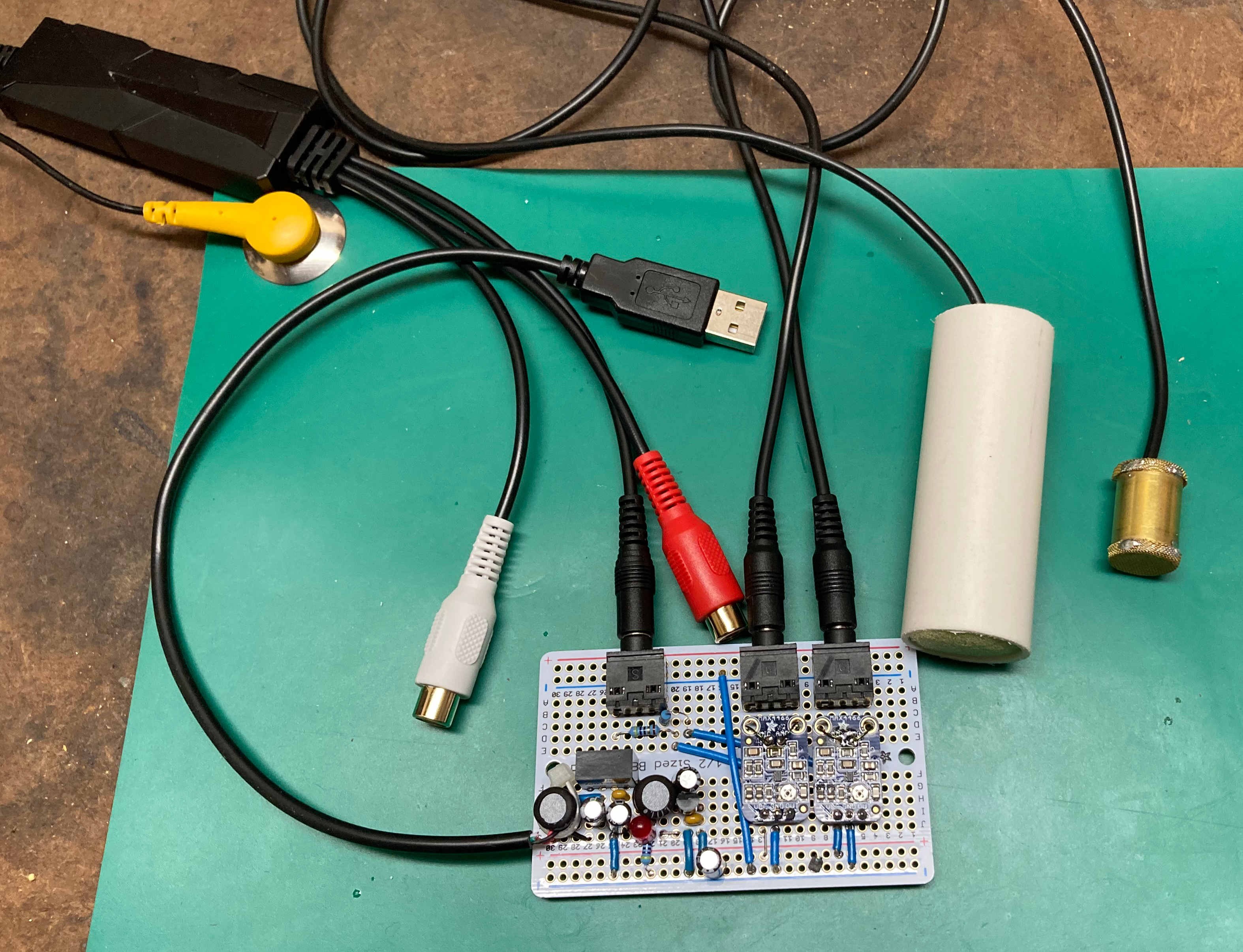
I picked a low cost USB capture sound card which takes an AUX "line in" signal (1V max) and samples both channels at 48kHz.  The Raspios Bullseye operating system did not need special drivers for the sound card so its use was plug-and-play.

Software

To minimize cost and size of the sensor, the base computer system was a Raspberry Pi 3B computer with Raspios Bullseye operating system.  Another economical element of this project was to use gnuradio as the software platform for signal processing.  Gnuradio has direct support for real-time audio sampling, signal processing, and useful display graphs.

The basic calculation is to perform a cross-correlation between the two sampled audio streams which produces an estimate of the time delay at the peak of the correlation function.  The calculation of cross-correlation is best performed using a Fourier transform and so the gnuradio flow-graph consists mostly of computing the FFT of both the left and right channel audio signals, multiplying them together, and then computing the inverse FFT of the result.  I picked a vector length of 8192 samples which at a sample rate of 48kHz generates a cross-correlation result every 171 ms.  The Raspberry Pi 3B has enough compute power to manage this calculation in real time, and display the correlation results in several graph formats including a rolling waterfall spectrogram style.

One discovery was that this calculation is sensitive to DC offset errors in the sound card samples so a DC block module is used in gnuradio to assure zero mean signals.

Another discovery was that in some linux distributions, including Raspios, the audio processing stream is first managed in the ALSA manager and then passed to the Pulseaudio server.  It turns out that pulseaudio can perform resampling and even sample-dropping, so because in this case where sample rate and channel sync are critical it is best to capture the audio stream directly from ALSA.  So the gnuradio audio source block points to a ALSA hardware capture device descriptor "hw:2,0".

Measurements

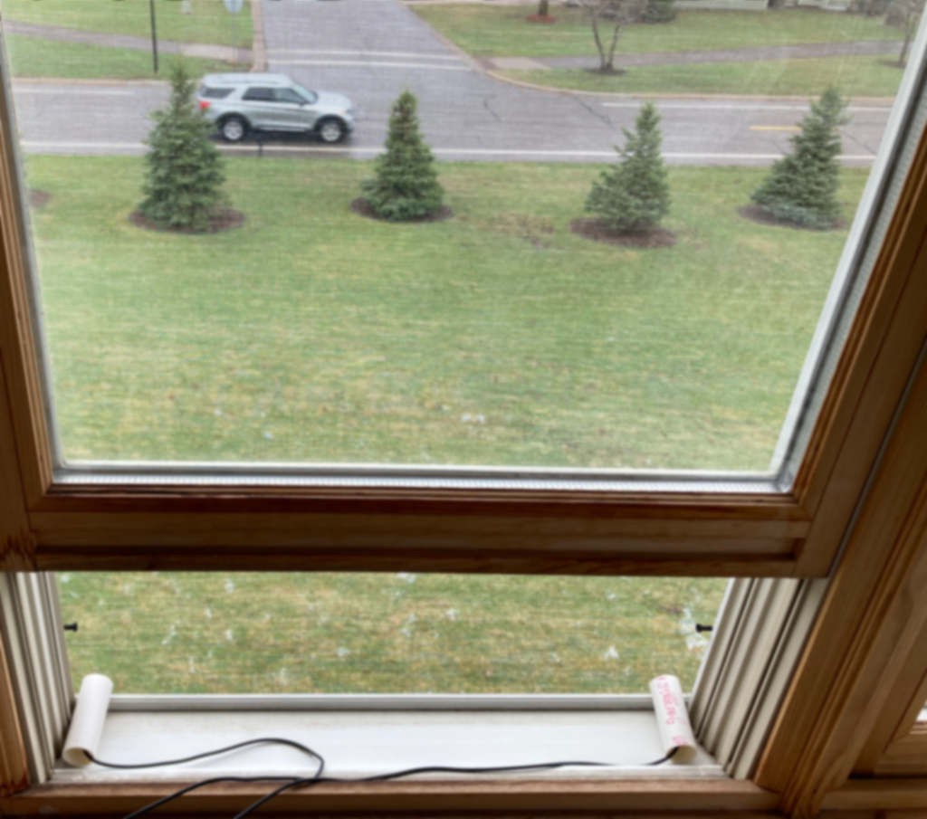
I placed the microphones in a window facing the street with a clear unobstructed view of the traffic.  The distance from microphone baseline to the road is about 33m.

The gnuradio flowgraph can save the correlation vectors to a file and I then displayed them using GNU Octave.

Figure 4 shows an example measurement of three automobiles moving past the microphone array.  It shows the full correlation map with delay sample along the horizontal axis and FFT vector along the vertical axis.  The blue areas represent zero correlation, whereas the green and yellow colors represent strong correlations.  Most of the useful information is in the center of the map where delay sample #4096 represents zero time delay.

Figure 5 shows a close-up of the same plot showing just the data in the center portion of the map.  This figure also shows the time delay units in msec across the top as well as the time of each FFT frame along the right axis which shows how the phase delay of the sound evolves as the vehicle moves in time.

Each vehicle shows a primary correlation pattern in the shape of an "S" curve as each moves from left to right or right to left past the microphones.  Each curve will follow the expression in Equation 1 above so the delay correlation may be used to compute the position and velocity of each vehicle.

Applications

This concept can be used to measure the presence and velocity of each vehicle passing the microphones.  For example, I measured delay correlations for a 71 hour period and generated a speed distribution for about 9000 vehicles shown in Figure 6.

This shows a mean speed of 34.5 MPH on a road with a posted legal limit of 30 MPH.  The measured traffic volume matches well the published traffic volume measurement of the municipal traffic engineers several years ago.

There are several limitations of this technique which I discovered in making these measurements:

• The sensors are vulnerable to interference from sounds other than the vehicles, such as car horns, lawn mowers, snow blowers, tree trimming, aircraft, dogs, birds, music players, etc.
• Weather will affect the measurement.  For example, the speed of sound varies with air temperature and so an accurate speed measurement will need to take air temperature into account.  Wind, rain, and thunder will produce sound interference.  Snowfall actually can quiet the sound of the vehicle tires on the roadway making measurement more difficult.
• There is a lower limit to the measurement of the speed of a moving vehicle as the sound amplitude drops as the vehicle slows.  This is also a benefit as the sensors will tend to ignore other quiet and slow moving objects such as pedestrians, skateboarders, bicycles, etc.
• There is an upper limit to measurement of the speed of the moving vehicle because the sensor produces only about 5 measurements per second and a fast moving vehicle will be undersampled as it passes by the sensor.
• It would be difficult to extend this concept to measure more than two lanes of traffic, i.e. more than one in each direction, since there would be significant overlap in signals from many vehicles at once, and the sensor would need to know which lane each vehicle is occupying.  So this concept would need to be extended to more than two microphones so that depth from the sensor could be measured also.
• The sensor array should have a clear line of sight to the roadway so that there are no significant reflections of the sound toward the microphones.  Each unintended reflection would superimpose clutter onto the delay calculation and mask the primary reception.