 wlf647
The finished project
What is an analog computer
Unlike a digital computer that represents numbers as sequences of 0s and 1s, an analog computer, for the purpose of this discussion, represents numbers as real-valued voltages. For example, the number 2.3 is simply 2.3 Volts at some point in the circuit.
Using op amps, we can build analog circuit elements that perform addition, multiplication, etc. on these voltages. We can also do more sophisticated things, like compute integrals over time, using an op amp integrator:
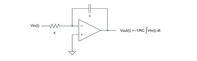
Imagine a physics simulation where we set the integrator input voltage Vin(t) to the speed x’(t) of a moving object. The object’s position x(t), which is x’(t) integrated over time, is then simply the op amp’s output voltage (scaled by -1/RC). In real-time!
Of course, modern digital computers outperform this ancient method in pretty much every way. But there is something beautiful and satisfying about solving problems with these minimalistic analog circuits.
The classic ball-in-box simulation
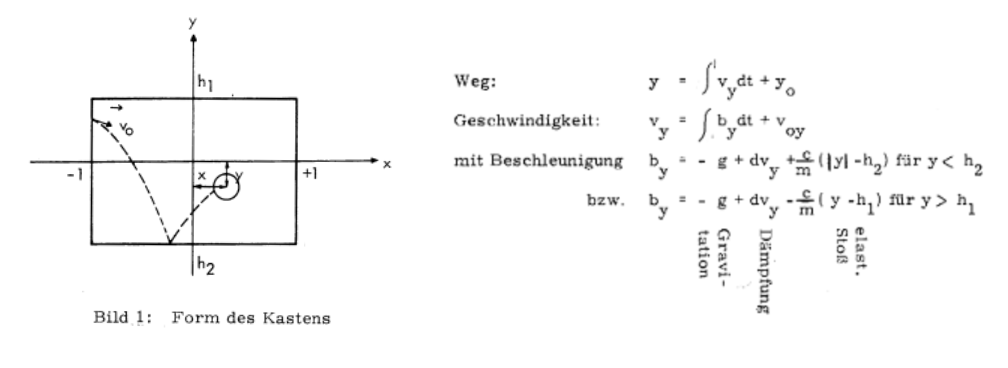
Computing the trajectory of a bouncing ball, subject to gravity and air drag, is a classic demonstration of what analog computers are good at. The German company Telefunken used it as a tutorial for their analog computers in the 1960s. Below is a screenshot of their “Ball im Kasten” (German for “ball in a box”) manual. The original document is in German, but here is a walkthrough in English.
A similar analog computer was used in the famous Tennis for Two demonstration from 1958. Like Telefunken’s “Ball im Kasten”, Tennis for Two was originally meant to show off the capabilities of analog computers. Remarkably, it is now considered one of the first video games ever created.
Today, the analog ball-in-box simulator still makes for a fun and rewarding electronics project. Here are a few implementations that are worth checking out [analogmuseum.org] [glensstuff.com] [hackaday2009], and here is a nice video of Eric Archer's build from 2009:
The goal of this project
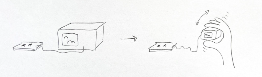
The goal of this project is to extend the classic ball-in-box simulator so that the user can pick up the physical “box” (the display), shake it, turn it over, etc., and watch the ball inside react in a physically plausible way.
To achieve this effect, we replace the fixed gravity term in the classic ball simulator with the readout from an accelerometer that is rigidly mounted to the display. The display needs to be small, of course, so that it can be easily picked up and moved around in space. A heavy oscilloscope will not work.
A small cathode ray tube (CRT) is a good fit for this project, since we can drive the beam deflection directly with the position of the ball (or rather, the position of the dot that draws the ball), using minimal circuitry. I decided to repurpose a vintage video camera viewfinder, a Sony CRT DXF-801, because it is small, there are many available on eBay, and I found a free schematic online.
The accelerometer is an ADXL335. It outputs three analog voltages proportional to its acceleration in three dimensions, which is the perfect interface for our analog computer.
Why this should work
To make the “pick up the box” metaphor work, we replace the constant gravity term in the ball simulator with live measurements from an accelerometer attached to the display, without any additional math. It may seem obvious at first that this works, but it is more nuanced when you think about it, since an accelerometer cannot distinguish earth gravity from acceleration caused by velocity changes of the display / box.
Proper acceleration is the technical term for what an accelerometer measures. The science here gets complex very quickly, at least for me. To convince myself that this hack should, in fact, work, I found it easiest to think about how an accelerometer works on the inside. Real physics people who read this: please go easy on me :)
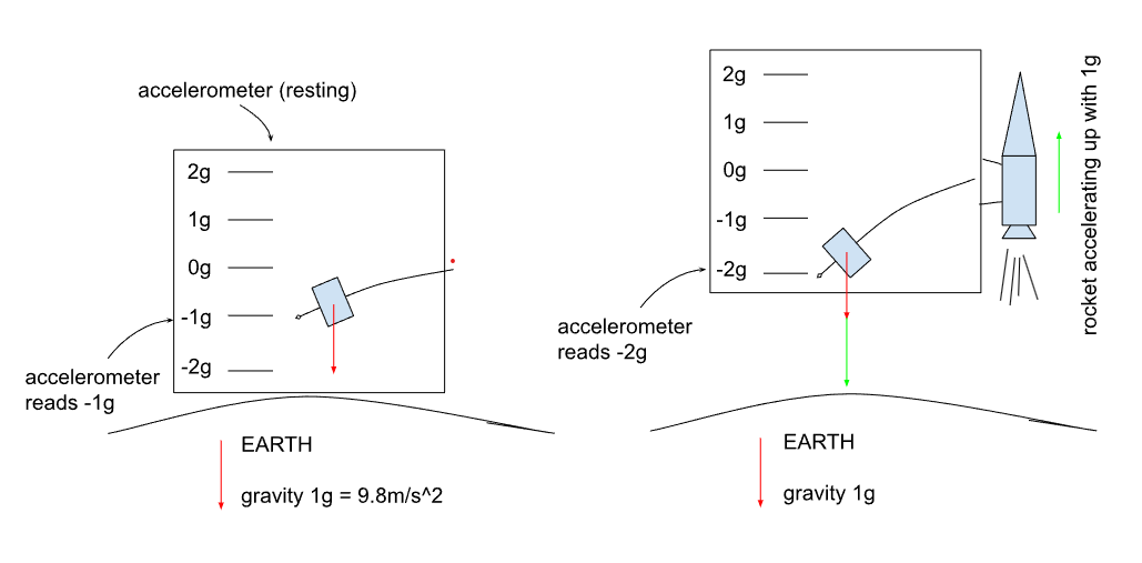
You can think of an accelerometer as a device that measures the displacement of a cantilevered weight, like in the diagram below. When the accelerometer rests on the ground (left picture), gravity pulls down on the cantilevered weight, resulting in a reading of -1g. If you now attach the accelerometer to a rocket and accelerate it up at 1g (right picture), the cantilevered weight is pushed back even more, and you get a -2g reading. Importantly, the accelerometer cannot tell what portion of the experienced -2g are due to its changing velocity vs gravity.
Why then does our simulation do the right thing, if we accelerate the ball with the raw output of an accelerometer? Let’s look at a few specific cases to appreciate why this should work:
First, assume the ball is in mid-air inside the box:
- If the box is stationary and upright, we have the traditional case which we already know works: acceleration is constant and points down, so the ball is accelerated downwards with 1g.
- Now when you pick up and move the box, the accelerometer reports the sum of earth gravity and that change in box velocity. But since the ball is in mid-air, the box acceleration shouldn't affect the motion of the ball. So to make the ball appear unaffected by the box movement, we have to accelerate the ball itself with the opposite acceleration to the box, which is precisely the delta the accelerometer reports!
The rocket example above helps illustrate this further: if the simulator display was on a rocket going up, the ball would now accelerate down with 2g, which to a stationary observer on earth looks like the correct 1g fall of a ball in mid-air, because the display itself, with the simulated ball on it, accelerates up at 1g.
What about when the ball is in contact with a wall? In our simulation, wall contact is modeled as a spring force. While in contact, the ball slightly penetrates the wall, and the wall pushes back like a spring.
- Imagine a flinging / launching motion, where we accelerate the box so that the wall moves towards the ball. During that motion, the ball will see a higher acceleration towards the wall that pushes it deeper into the wall. At some point near the end of the flinging motion, the box acceleration decreases, and the wall now pushes back harder than the ball is pushing in. This launches the ball off from the wall, as we would expect.
- Finally, imagine the opposite motion, where we accelerate the box so that the wall that the ball rests on moves away from the ball. Again using the cantilever weight metaphor, we can appreciate that this acceleration pushes the ball away from the wall. If it exceeds the acceleration that pushed the ball into the wall in the first place, the ball will separate from the wall and start moving away from it, as we would expect.
I hope this helps. Please check out the demonstration video to see the system in action. I do believe that it does in fact do the right thing. Any feedback on how to explain it better is welcome.
Thanks for reading!