It is done! In today's update I will discuss the finished product (finished meaning for the hackaday op amp challenge, ideas for future work are listed below). I have a demo video of the system working and some deeper insights into how component values were picked and how the bounce logic works. I also finally wrote the high-level “Why this works” part in this project’s Details section.

Attaching the accelerometer to the display

As the final build step, I have replicated the accelerometer circuit on a protoboard and mounted it to the handheld CRT display. I 3D printed a rectangular frame to hold the protoboard and stuck it to the side of the display housing with double-sided tape. 

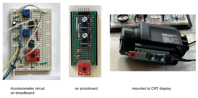
The accelerometer is deliberately positioned close to the front of the display, where the screen is. That way, we always measure linear acceleration on the side of the housing where the simulated “box” is. The placement of the accelerometer wouldn’t matter if we only allowed translational movements or very slow rotational movements of the display. But it is unavoidable in practice, and quite fun actually, to “wiggle” the display (e.g. quickly tilt it up and down) to move the ball around. During these fast rotational movements, measuring linear acceleration at the back of the case would yield the opposite of what we expect to see on the front side where the ball is displayed.

The finished system

Random side note: I’m kind of proud of this technique I came up with for making a scrappy cable assembly with .1” header connectors and strain relief in a hurry: just cut a paddle-shaped support plate out of 2mm ABS and superglue the header and outer cable jacket to it. Works great :) 

Demo video

Without further ado, here’s a video of the system in action. Make sure you have sound on, I find that the sound effect nicely adds to the illusion. I’m super happy how well this circuit performs! 

Double-checking our simulation parameters

The motion equations for the ball are independent for each dimension (x and y) in our 2D simulation. Each dimension is modeled with two op amp integrators and four passive components, as shown in the schematic snippet below. The circuits for x and y are identical.

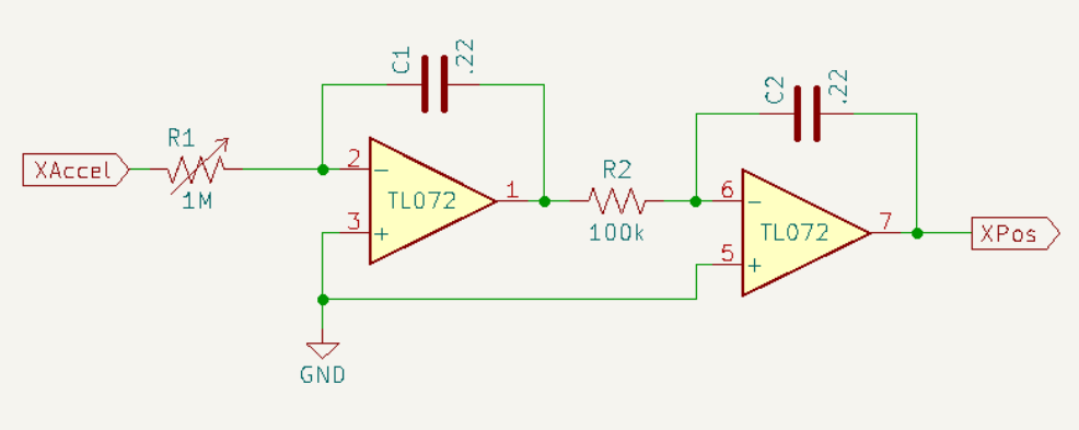
Note that this is for ball motion without wall collisions. We look at the bounce logic in the next section below. 

I chose the values for R1, R2, C1, C2 by trial and error, such that the simulation “looked right”. The shown values R1=100k, C1=C2=.22u worked well, and I found it useful to leave R1 variable, to control how strongly the ball is affected by inputs from the accelerometer. Around 120k felt pretty good for R1.

But since we are measuring actual earth gravity and acceleration of the box, there should be a “correct” choice of parameters. Let’s do the math and see if the above values make physical sense.

Let’s use a(t), x(t) to describe acceleration and position in the real world, in meters, and v_a(t), v_x(t) to describe the corresponding voltages in our simulator. Here is the equation that relates acceleration to position in the real world

Our simulation circuit in the schematic above implements

How do v_x (t) and v_a(t) relate to x(t) and a(t)? 

1. v_x to x: the display is 2x5.1V “wide” in our simulator and 28mm wide in the real world, so x / v_x = 1m / 364V, or x = (v_x / 364V) * m
2. v_a to a: our accelerometer + signal conditioning produces about 1V per g, so we have a / v_a = (9.81m / s^2) / 1V, or a = (v_a / 1V) * 9.81m / s^2

Substituting these relationships into the real world formula we get

Dividing by the 1/V and m units, and combining constants, we get 

Now we can compare coefficients to the integral equation of our simulator circuit, and find that 1/R1C1R2C3 must be 3574/s^2. The s^2 units checks out, because RC is in seconds, so RCRC is in s^2.

In our case, with C1=C2=.22u and R2=100k, what value does R1 need to be? It's 3574 * (.22e-6 *.220e-6 * 100e3) = 58kOhm!

Again, the value I picked experimentally to make the simulation look "right" was 120k. It about twice the theoretical value. But that's not too far off, considering part and measurement tolerances, and how closely you can expect to even judge physical correctness on this crude display. 

One more interesting thing to note is that when the value of R1 is off, both earth gravity and accelerations caused by box movements are equally off. So if we wanted to simulate low gravity, we can't just make R1 large. I found the most convincing way to play with low gravity is to simply hold the display vertically (screen parallel to the floor). Then, earth gravity has no effect, but box acceleration affects the ball as before.

Deep dive into the bounce circuit

The bounce logic is shown in the inside blue box below. The op amp to the right is the first integrator of the motion equations we just discussed above. It takes the sum of the accelerations from the accelerometer (through R25) and from the wall bounce (through R26), and integrates them into the (negative) ball X velocity. 

There are four bounce circuits like this, one for each wall of the box (or side of the display). The one shown here is the left wall and it works like this. 

• While the ball is to the right of the left wall, XPos > VRef- (-5.1V), and the op amp output is at -100 x (-5.1V - XPos), which is likely at the negative supply rail, -7.5V. In that state D8 is reverse biased, so no current flows through R26, no bounce acceleration.
• When the ball crosses the left wall, the op amp output goes positive, 100 x the penetration depth. Now, D8 is forward biased and a bounce acceleration is applied to the velocity integrator through R26. 

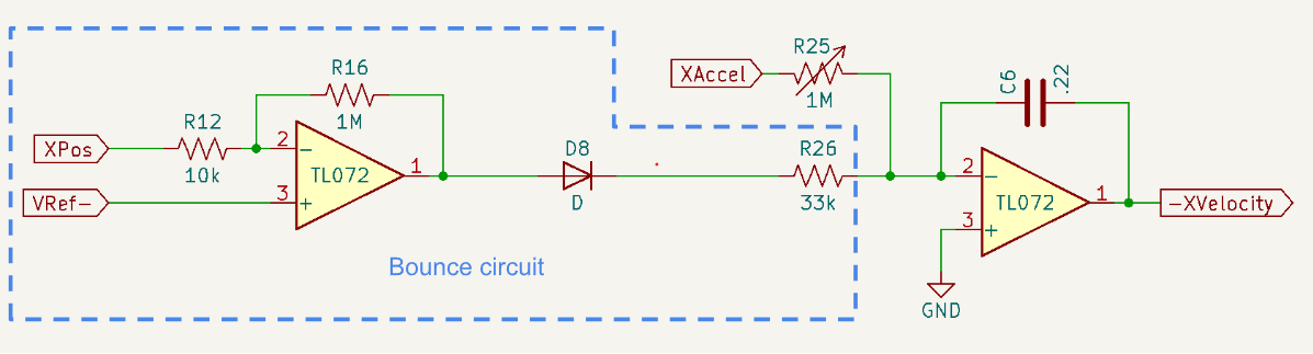
Effectively, the wall is like a mechanical spring (F = -kx) with spring constant k = 100 (R16/R12) that accelerates a ball mass proportional to R26. 

I picked the resistor values as follows: I wanted a large R16/R12 ratio, so I made R12 small (10k), but not too small where it would present a significant load to the preceding circuits, and R16 large to get a strong bounce (1M), but not too large where the op amp output would saturate too often, as shown in the scope traces below.

While picking R26, I ran into some practical limitations of the circuit that are worth discussing. 

In theory, if the wall acted like a perfect spring, the ball’s velocity would be exactly reversed during a bounce. The only thing that R26 should change is how “squishy” the bounce is. Larger R26 means larger ball weight, so the ball penetrates deeper into the wall and takes longer to reverse its velocity. So I expected that changing R26 would be a matter of just picking what looks best.

Instead, here is what I found 

1. Regardless of the bounce resistor values, there is always a substantial amount of damping present in my circuit, i.e. the ball always loses some energy with every bounce. Of course, some amount of damping is desirable for our simulation, since that’s what happens with a real ball as well. But it’s not obvious where damping happens in the circuit. 
2. Changing R26 did not only change the “squishiness” of the bounces, but also significantly affected the amount of damping: the least amount of damping was for R26 around 100k. Both decreasing and increasing R26 from there, resulted in more damping. 

Here are scope traces for different values of R26 and an attempt to explain R26’s effect on damping. The traces were produced by holding the display with the bottom right corner pointing towards earth, then quickly rotating the box counter-clockwise so that the bottom left corner points down. This makes the ball fall along the full screen width down to the left wall. Here is the first experiment with R26 = 1k:

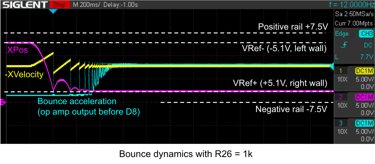
You can see the damping in the ball height (magenta) reducing with each bounce. The bounce acceleration (cyan) comes in very short spikes that reverse the ball velocity (yellow), until an equilibrium is reached where the bounce acceleration exactly cancels out the gravity pushing the ball into the wall. 

Here is what happens as we increase R26:

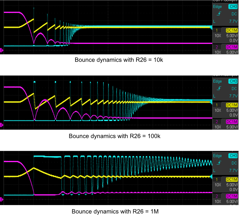
A few observations: 

• The minimum damping (highest bounces, magenta curve) occurs with R26=100k.
• As expected, larger R26 values make the bounces squishier, so 
• bounce events take longer (wider pulses on the cyan trace), 
• the ball pushes further into the wall (lowest point of magenta curve is at -5.1V for R26=1k and goes all the way down to the negative op amp rail for R26=1M)
• As the ball pushes deeper into the wall, the bounce op amp output saturates a lot (cyan curve goes to top rail). 

Here is how I would explain the damping depending on R26 values. I’m not super confident about this, so I’d love to hear your thoughts:

• For large R26, both the position and bounce op amps outputs go to the rails, so our physics model is no longer valid. For example, during the first bounce with R26=1M, the ball hangs out at an artificially shallow depth, with an artificially low spring force. By the time it leaves the wall, it has barely picked up any of its initial motion energy.  
• For small R26, the bounces are simply too short and we are limited by the bandwidth of our simulator. My guess is that in R26=1k example, the velocity has to change so quickl that the circuit simply can’t keep up, due to parasitic capacitances, slew rates, etc. 

The value I ended up picking for R26 is 33k. It felt like a good compromise between squishiness and damping. 

When you look at other ball-in-box implementations, you will sometimes see a “bleeder” resistor across C6, which is a way to implement damping more similar to air drag. I did experiment with this approach, but probably due to the bounce-related damping effect we just discussed, I didn’t find the bleeder resistor effective. Of course, it would be nice to be able to model damping during bounces more explicitly, rather than taking advantage of limitations and parasitics in the circuit. But that’s for a future project :) 

Future work

I wanted to build this project for a while when the hackaday op amp challenge finally prompted me to actually build it. I’m happy that I got it working just in time! I’m going to take a break, but there are some things I’d like to get back to in a bit.

One thing that I didn’t get to do was really characterize and understand the CRT coil drive circuit. The resistors R43/R44 removed the ringing I saw initially, but also did occasionally see what looked like further stability issues (oscillations?). There is some good information on making compensation networks for deflection coils in this application note: https://www.apexanalog.com/resources/appnotes/an05u.pdf 

Originally my plan was to build this on a PCB, but I ran out of time. I’ll probably still do that, since it’s a cool demo I’d like to keep ready to go after I clear my breadboard for other projects. 

Thanks so much for reading!