 Joan Horvath
Calculus is all about figuring out how something is changing (or how it has accumulated changes to this point). There is a lot of terminology with this that scares people off… derivatives, differential equations, integrals … but the concepts that these are shorthand for are not all that hard. We want to make this readable for people who have never seen these concepts before, and make it possible to find more online. When we define a word we think you'll want to know more about later, we'll make it a link so you can can go and read more elsewhere if this is all new to you.
The ideas apply to all kinds of changes, like pressure going up or down in a gas or stock prices rising and falling. But Newton mostly talked about actual, physical motion. Since that’s the easiest to think about for most people, that’s what we will talk about here.
Our next build (in the next few logs) will be a mechanical device that will let you graph how something is changing, which calculus would call the derivative. The process of calculating a derivative is often called differentiation. This log ties together the acceleration detector in Log #1 and our “mechanical differentiator” that we are working on in the next few logs. Later on, we are going to figure out ways to use 3D prints to visualize more complicated systems. But for now, we will go back to some very basic stuff.
Slope of a Curve
Imagine that you are running somewhere and that you always run at the same speed. You might go a tenth of a mile in a minute, have gone two-tenths in two minutes, and so on. Your distance traveled would look like this, but your speed is constant (because we said to walk that way) as we draw in the graph that follows:
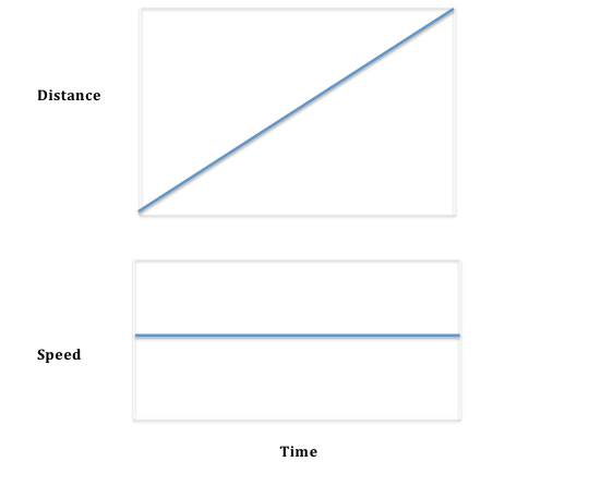
If we asked you how fast you were running you might say “a tenth of a mile per minute” or maybe “six miles per hour.” This is the change in distance (a tenth of a mile) per change in time (a minute). Mathematicians would call this the slope of the line in the first picture – or, alternatively, the derivative of the curve in the first picture. In this case (constant speed) the slope of the whole curve is a constant and the derivative is a straight line. Let’s visualize when they are not, which was where Newton pulled together some old and new insights to create some powerful tools.
Instantaneous Slope
The example above is so easy that you are probably rolling your eyes. But suppose that the curve isn’t so simple. Look at these next two animations (done in OpenSCAD).
Notice the little line moving along the top curve. That is the instantaneous slope of the curve (it is also a line that is tangent to the curve). The bottom line is the value of that slope, just like our previous graph in this log. The little line on the bottom curve is showing that the slope is calculated from the past and current behavior of the top curve. We can't talk about change of a curve without having at least two points, although we want those points to get closer and closer together to make the slope more and more instantaneous. (There are many ways to calculate slope, but just think of this simple two-point way for now).
This first example is what it would look like if someone started out away from their house, and moved toward it and past it such that their velocity increased as shown in the lower graph. (Negative velocity we will interpret as toward the house, in this case). At the minimum point they arrive at the house, then move away again. The distance (the top line) is then a parabola.
In this next case, someone is running back and forth, say to the right and then the left of a starting point, with their speed varying in a way we call a sinusoidal wave. The slope of a sinusoid is another sinusoid, offset in time (and sometimes scaled bigger or smaller.)
Newton’s big insight was that if he looked at the instantaneous slope on a complicated curve (how the curve is changing if we drew a shorter and shorter slope line) he could come up with a way of describing (and then analyzing) the speed of anything, once he had a graph of how the distance varied versus time.
He was interested in how the planets moved, and he had a lot of data that had been taken by his friend and editor Edmund Halley and the earlier astronomer Tycho Brahe, plus some rules that seemed to predict planetary orbits from Copernicus and Johannes Kepler. So he had a lot of distance versus time measures (that he still had to interpret without knowing for sure how Earth was moving relatively).
Acceleration
We don't have to stop with the slope of a curve. We can take the slope of the slope- how fast our speed is changing. This is called acceleration if we are talking about motion, and in general the second derivative (the slope of the slope of a curve.) You can keep going - the third derivative is sometimes called "jerk" and is something that 3D printer designers worry about a lot.
Trying Things Out
If you take the device from log #1, you can see acceleration in the plane of the board (it ignores anything perpendicular to the board.) The red lights will "slosh" to points with more and less acceleration. Try moving your hand in a way that matches VELOCITY to the DISTANCE curve here. You can watch the brightness and direction of the red lights and think about how they are showing the derivative of the speed (not distance) of your motion.
The Mechanical Differentiator
We thought about 3D printing curves and surfaces and their derivatives, and we will set up some of that in later logs. But first, we thought a mechanical way of running a device along a curve that could draw its derivative curve would be useful. We were sure that there must have been such devices in the pre-computer era, since there are very practical applications. There sort of were; in the upcoming logs about the design process we will talk about some of them. Open-source hardware like that used for 3D printers makes assembling such a thing a lot easier than was possible in 1916, when one of the more elegant designs came along.
Discussions
Become a Hackaday.io Member
Create an account to leave a comment. Already have an account? Log In.