 Bruce Land
The plan here is to build up intuition for HiD representations in parallel coordinates:
- points -- The basic representation of points as lines in PC.
- lines -- The observation that lines map to points in PC.
- planes -- Hyperplanes can be detected visually.
- clusters of points and random distibutions.
- polytopes (HiD polyhedra) using envelopes and line-density plots.
- dynamic systems using an extrusion scheme.
Examples
- 3D Points in parallel coordinates.(matlab code)
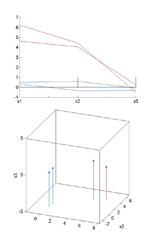
![]() Each of the four 3D points becomes two line segments in PC. This projection
onto parallel lines maintains most of the geometry, but in different form.
Each of the four 3D points becomes two line segments in PC. This projection
onto parallel lines maintains most of the geometry, but in different form. - Cluster in 3D (matlab code)
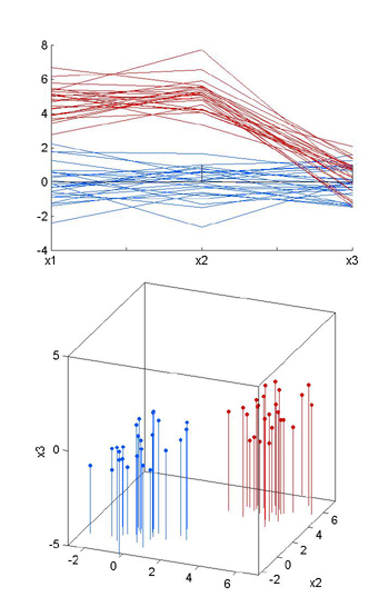
![]() The two clusters shown are separated along the x1 and x2 axes, but not on
the x3 axis. The cluster centers are [0,0,0] and [5,5,0].
The two clusters shown are separated along the x1 and x2 axes, but not on
the x3 axis. The cluster centers are [0,0,0] and [5,5,0]. - A 2D cluster (matlab code)
![]() Two 2D clusters are shown in the middle panels. The left one is filled from
about 50% to 100% radius. The right one from 10% to 100%. The top panels are
the PC plots. There is visible difference between the two, but hard to see.
The color code for the top two panels are color by distance of the point from
the origin. The third panels are coutour plots of the density of lines in the
PC plots. There is a clear difference between the hollow cluster and the solid
cluster. The color code in the bottom panels is density, blue low, red high.
Two 2D clusters are shown in the middle panels. The left one is filled from
about 50% to 100% radius. The right one from 10% to 100%. The top panels are
the PC plots. There is visible difference between the two, but hard to see.
The color code for the top two panels are color by distance of the point from
the origin. The third panels are coutour plots of the density of lines in the
PC plots. There is a clear difference between the hollow cluster and the solid
cluster. The color code in the bottom panels is density, blue low, red high. - A line in 3D. (matlab code)
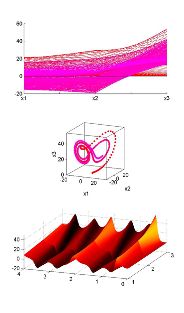
![]() The line segment x1=t; x2=1-.5*t; x3=0.5-.1*t; with 0<t<1 is drawn
in normal 3D coordinates and in PC. The color is relative t value. Note that
each point on the line becomes two line segments in PC (x1-to-x2 and x2-to-x3).
The obvious convergence of all the line segments between the x1 and x2 axis
is a direct consequence of the linearity of the points and partly defines
the line. A less obvious convergence of line segments to the right of x3 completes
the definition of the line.
The line segment x1=t; x2=1-.5*t; x3=0.5-.1*t; with 0<t<1 is drawn
in normal 3D coordinates and in PC. The color is relative t value. Note that
each point on the line becomes two line segments in PC (x1-to-x2 and x2-to-x3).
The obvious convergence of all the line segments between the x1 and x2 axis
is a direct consequence of the linearity of the points and partly defines
the line. A less obvious convergence of line segments to the right of x3 completes
the definition of the line. - A plane in 3D (matlab code)
![]() The middle panel show a plane in 3D space. The plane is given by
The middle panel show a plane in 3D space. The plane is given by - A dynamic system plotted as a surface with PC and time as axes (matlab
code)
![]()
- A 2D line is rotated through 180 degrees (matlab code). The animation shows that a rotation in cartesian space...
Such a plot rapidly gets cluttered with a large number of lines. If you squint at the PC plot, you get the feeling that density of lines might be important for determining the center of the cluster. The next plot shows an example of distinguishing cluster shape by computing line densities.

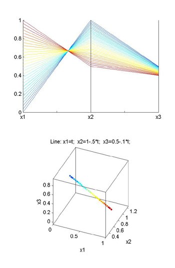
If the slope of the line relating one axis to another (e.g x1 to x2) is m
and the intercept is b in normal coordinates, then the position
of the convergence in PC is the point
[ 1/(1-m) , b/(1-m) ],
asuming that the first axis (x1) is located at horiziontal position zero and
x2 is located at horizontal position 1. For the line given above the slope
from x1 to x2, m=-0.5 and b=1. Thus the first convergence
point should be [0.67, 0.67] as shown.
The slope from x2 to x3, m=0.2 and b=0.3. Thus the
second convergence point should be [1.25, 0.375], or just to
the right of the x3 axis.
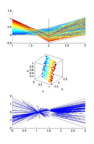
x1= t
x2=-.5*t+.5*u
x3 = 1.1*u
Where t and u are uniform random variables from 0 to 1. The color code is proportional to t.
The top panel shows the PC representation of the plane. There is clearly structure to the points, but it hard to see what it means, except of course that the color mapping is along x1.
We would like some way to detect a plane by a visual technique. The bottom panel shows one of two characteristic points of this plane plotted in PC according to the following scheme. Pairs of points in the plane define lines in the plane. For a large number of pairs of points (lines in the plane), compute the two points in PC which describe each 3D line (in the plane) as in the example above then connect them with a line. If all the constructed lines pass through a point, then the points fall on a plane. If the plane were noisy, then the lines would 'almost' pass through a common point.


 Keith
Keith
 Kwabena W. Agyeman
 Ted Yapo
Delighted that you liked Parallel Coordinates (||-coords) and the Altruisms motivating to continue. BTW see the 2009 book (Ch.9) for neat ways to draw curves and hypersurfaces not pt by pt. Many thanks and congras