 peter jansen
I happen to think that magnetic resonance imagers, or MRIs, are one of the most incredible machines that humans have built -- right along side spacecraft and large hadron colliders. MRIs are volumetric imagers, which means that they can scan inside objects and produce very accurate three dimensional renderings of where certain protons are, like the protons in the two hydrogen atoms that make up each water molecule.
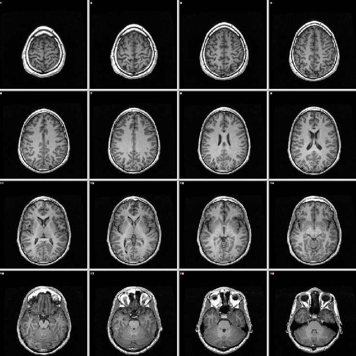
I confess that I didn't have a full appreciation for just how incredible MRIs are before taking an Advanced Brain Imaging class in graduate school, about six or seven years ago. Before hand I was largely only familiar with the common structural images that MRIs take, like the ones of my brain (above) often for diagnostic medical imaging like locating tumors or characterizing trauma. In cognitive neuroscience, we also made use of functional magnetic resonance imaging (fMRI), which is able to help identify the brain regions that are active when someone is completing particular tasks by measuring areas where there is increased blood oxygenation (the so-called BOLD signal). But it turns out that MRIs are capable of many more incredible methods of imaging. Magnetic Resonance Angiography can map the blood vessels in the body, Diffusion Tensor Imaging (DTI) can help image the neural connections in the brain, Magnetic Resonance Spectral Imaging can measure metabolic changes in tissue, to name only a few of the incredible techniques available. Even with all these incredible techniques, the structural images are still beautiful, and I really enjoy seeing structural scans of everyday objects, like these scans of fruits.
Magnetic Resonance Imaging (MRI) and Computed Tomography (CT)
Ever since taking that Advanced Brain Imaging class I've been thinking about how one might go about constructing their own MRI. It's not an easy task (we'll see why in a moment), but first let's look at a related imaging technique -- computed tomography (or CT) scanning. CT scanners are essentially x-ray scanners that are rotated 360 degrees around an object, and using reconstruction techniques like filtered backprojection, one can back out 3D information from a large number of 2D absorption images taken at a large number of different angles around an object.
 A little over a year ago I built a prototype desktop CT scanner, using a 10uCi Barium-133 radioisotope check source as a source for x-rays, and a modified extra sensitive Radiation Watch Type 5 high-energy particle detector to sense these low-energy x-rays. The first images of produce were really exciting for a first pass at a home built scanner, like the bell pepper below:
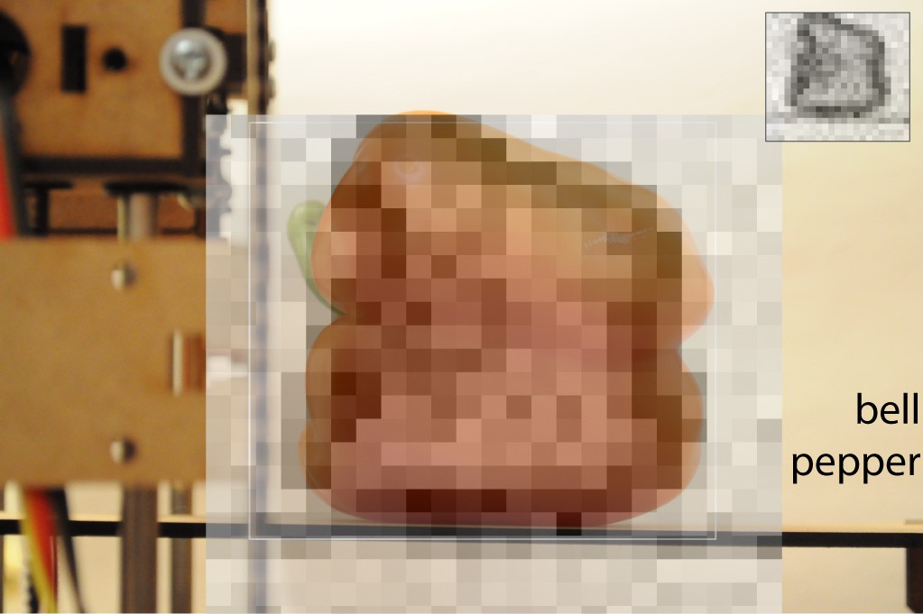
Unfortunately, these images took a good deal of time to acquire, because of the low intensity of the source. At about 90 seconds of sample time per pixel, a ~20x20 image took all night (about 10 hours) to acquire, so doing this at 1 degree increments would mean it would take an impractically long amount of time -- about 2 months -- to collect enough data for a 3D reconstruction. This is using the most intense radioisotope source that's legally allowed to be purchased, with a detector paired to be particularly sensitive to it's emissions. To speed this up you could add parallel detectors for a linear gain (ie. 10 detectors would reduce the scan time by a factor of 10, to 1 hour per slice), or increase the intensity of the source by using an x-ray tube. As a scientist it's important to be incredibly responsible, and one's health is just to precious to place in genuine danger with such things (not to mention the legal issues that undoubtedly exist). That leaves few options for CT scanning -- either find another wavelength, or decrease the source-detector distance, and construct a bank of tens of detectors to reduce the scan time to something on the order of a day. I'd thought about doing exactly this (the prototype is sitting beside me!), but really I'm at the mercy of inspiration, and what really inspires my volumetric imaging interests is the idea of figuring out a way to build an inexpensive desktop MRI.
The basics of Nuclear Magnetic Resonance (NMR)
Prefacing this by saying that I'm only an interested amateur and not an expert on MRIs or NMRs, so you'll have to forgive the vast oversimplification, but the MRI can be though of as an imaging extension to a nuclear magnetic resonance spectrometer. Nuclear magnetic resonance suggests that we can think of different nuceli as atomic-sized magnets. When in the presence of an external magnetic field, some portion of those nuclei tend to align to be in the same direction as that external magnetic field. When in this state, they become susceptible to absorbing and emitting ratio waves under certain conditions, and an NMR (and MRI) capitalizes on this by placing an object in a large magnetic field so that some portion of its nuclei will align to that field, broadcasting specific patterns of ratio waves into the sample, then listening to the radio waves that return. These radio waves can describe the atomic makeup of the sample (spectroscopy), the location of different parts of the sample (imaging), or the magnetic field intensity in the sample (magnetometry).
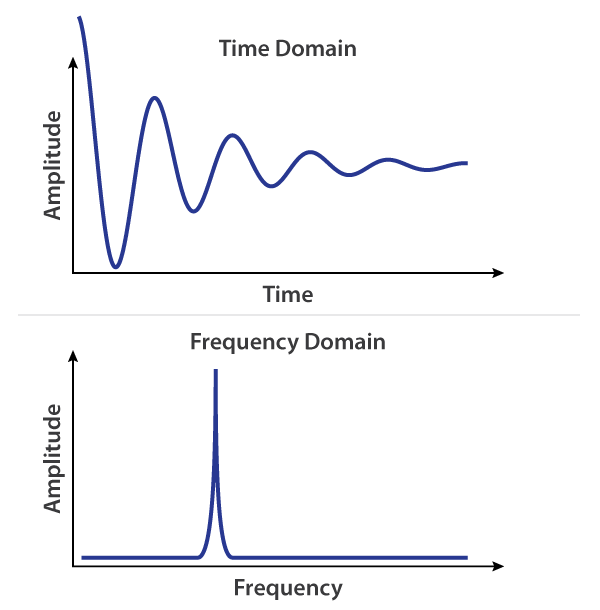
The simplest case, that I've animated below, is the Proton Precession Magnetometer (see the great PyPPM by Bradley Worley, or Signals from the Subatomic World on Amazon, for much more detailed information). Here the compass needle represents the orientation of the magnetic field of a nuclei, which starts out aligned with the orientation of a low-intensity ambient field, here the ~40 microTesla (uT) field generated by Earth's iron core. If the nuclei is then exposed to a much larger external field, say from a large electromagnet, it will shift and align it's orientation to that much larger field. If that larger field is then switched off, the nuclei will re-align to the Earth's field, slowly precessing back and forth until it has realigned to the lower field. This motion is defined by an exponentially decaying sinusoidal wave, whose frequency is defined by the Lamour Frequency, and can be picked up by an external antenna near the sample. The frequency varies with the strength of the magnetic field -- for Earth's low intensity field the frequency is only about 2kHz (audio frequencies), where as for a 1 to 3 Tesla medical MRI scanner, these frequencies are in the 40-100MHz range.

From the perspective of our receiver, we would observe the following exponentially decaying sinusoidal signal, and it's frequency, which can tell us the precise magnetic field intensity that the sample is in. The frequency variation (ie. the width of the peak in the frequency graph) can determine how homogeneous -- or how much intensity variation -- there is in the magnetic field. Traditionally, the more homogeneous the field, the more resolution one can get out of their instrument -- spectral resolution in the case of the NMR, and spatial resolution in the case of the MRI.
Because of the complexity of pulse sequences and the field homogeneity requirements, we're keeping things simple and aiming for creating (essentially) an imaging proton procession magnetometer, with a pulsed main field.
Extending NMR into an imaging technique
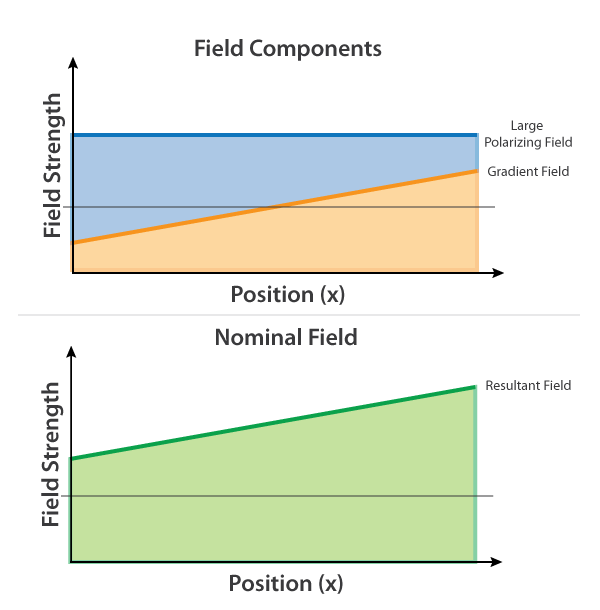
The frequency that a given sample will oscillate at depends on the intensity of the magnetic field that it's experiencing, and MRIs make use of this by introducing a slight gradient in a large main field. Where the large main field (say 1 Tesla) coming from a superconducting magnet is in blue, a much smaller gradient field (orange) emitted from a gradient coil introduces a very slight variation into the field, resulting in the sample experiencing the field in green.
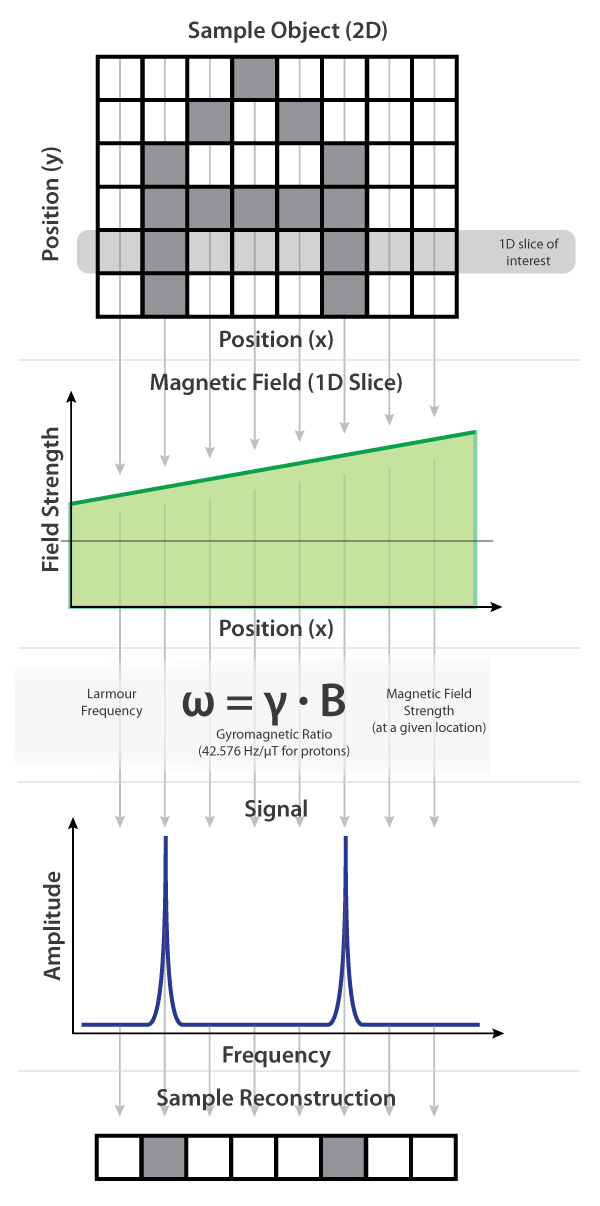
Because different parts along the length of the sample experience slightly different fields, the frequency that they emit at will be of slightly different frequency. Knowing the field intensity and gradient very precisely ahead of time allows us to back out exactly what location a signal at a given frequency came from. If a large signal occurs at that frequency, we plot the pixel as (say) dark to indicate the presence of signal, and if no signal occurs, we plot it light to indicate the absence of signal.
To help ground this in a 1D case, the figure below shows a single 1D slice of the letter "A" being spatially coded using a gradient field, the two locations where there is sample (x=2 and x=6) each transmitting at specific frequencies defined by the Larmour Frequency of the field intensity at their respective locations, and the reconstruction that can be generated by remapping the intensity of the signal at a given frequency back into spatial data.
Coded Aperture (or, "Coded Field")
The trouble with all of this is that superconducting magnets are fantastically expensive, and out of reach for building ones own MRI. NMRs can make use of large electromagnets that have much higher field inhomogeneities, but in order to do this they physically spin the sample around within the field so that the sample receives the "average" field intensity, but that doesn't translate well to spatial imaging.
A few years ago I did my first postdoctoral fellowship in computational sensing focusing on something called coded-aperture spectroscopy. Coded aperture spectroscopy doesn't have a good online tutorial that I can link to, but the heart of the technique is that instead of making a spectrometer that looks like a camera (where it's detector would make a high-fidelity representation of a spectrum), it places a special filter somewhere in the imaging plane so that the image on the detector looks nothing like the spectra, but the signal has been manipulated so that different kinds of inference are much easier.
In the extreme case, a linear CMOS sensor in a traditional spectrometer might be replaced with a single pixel photodetector in a coded aperture system, so that the entire spectrometer outputs only a single number per measurement cycle. At first this sounds crazy, but by changing the filter pattern on the coded aperture, you can actually target the spectrometer to do certain kinds of tasks extremely quickly (like spectral classification -- or identifying which chemicals are in a sample), and in many cases this can be done in orders of magnitude more noise than a traditional spectrometer. It's really an incredible technique.
An imaging analog to this is the Rice Single Pixel Camera, which contains only a single photodetector, but is able to take images through the use of an adaptive coded aperture. In the case of the single pixel camera (and the spectral imagers that I worked on), the coded aperture is usually implemented using a micromirror array, like those used in modern DLP projectors. By taking a variable number of measurements with different codes, one can back out what the original signal looked like, or use the signal for some specific purpose (like a spectral classification task, in the case of spectroscopy, or image identification, in the case of imaging). Surprisingly, a lot of work has been done with random codes, which work reasonably well for some tasks -- but you can also design the codes using various techniques, and this ultimately reduces the amount of measurements that you need to take for your task.
The interesting thing about considering MRI with an inhomogeneous (to a degree) electromagnet, is that it starts to conceptually look very similar to coded aperture spectroscopy and imaging. And as long as you can measure the field inhomogeneities over the sample region of the instrument (the 3D "code", in the form of magnetic field intensities and orientations) to a reasonable degree, and manipulate them, then I believe you can use the same coded aperture techniques to back out spatial data when using an electromagnet.
An example
Returning to our example from above, we can substitute in an inhomogeneous but known field (purple) instead of the very precise gradient field from above (green). Now, instead of there being a linear correspondence between spatial location (x) and frequency, the mapping is more complex. In this simple example, spatial location x=1 now maps to the second frequency bin, location x=2 maps to the fourth frequency bin, and because the field intensity is the same at different locations, multiple spatial locations pool their signal into the same frequency bin. So the measurement that we take (the signal in frequency space) looks nothing like the high-fidelity representation of the slice of interest that it used to -- instead we have to add in an extra step that uses our knowledge of the field inhomogeneities (the "code") to back out what the original slice looks like.
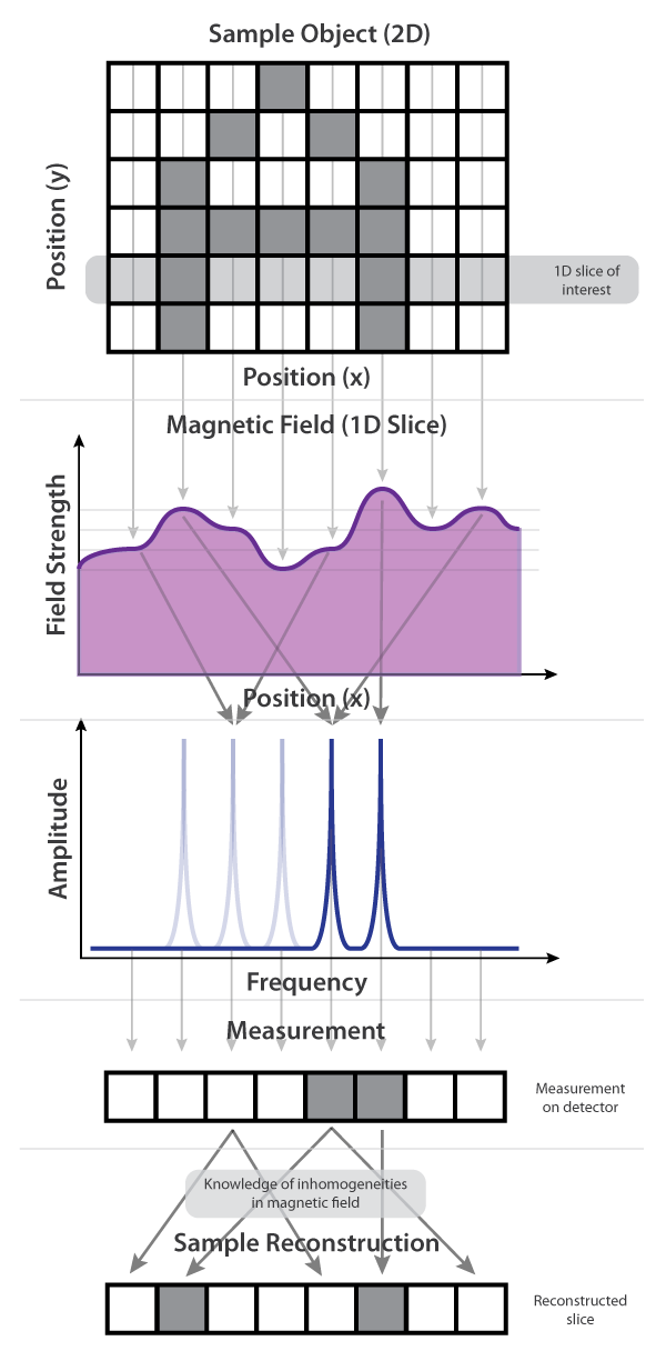
And because multiple spatial locations may share the same frequency bin (for a given code), we have to measure the same slice using a number of different codes to properly reconstruct the original slice. Generally the more codes that are used, the more accurate the final reconstruction will be -- although instead of using random patterns on the codes, you can design the codes using different techniques to decrease the number of measurements that are needed (relative to random codes) for a given reconstruction accuracy.
Below are two examples of codes -- the first one is the same as we just saw (above), and the second one is another random code with a different spatial mapping. We can also approximately represent these codes as discretized 1D images, as below, where the field intensity of the code at a given spatial location is represented by the intensity of the pixel at that spatial location (here, darker means a more intense field).
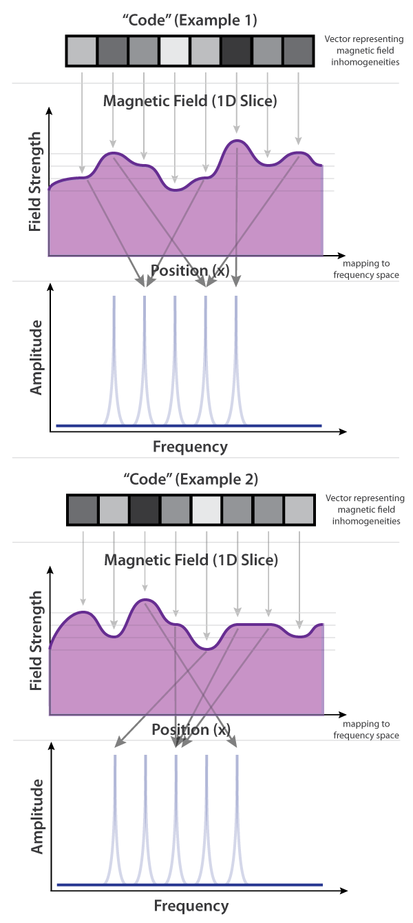
And these are only two examples -- in practice we'll likely need tens or hundreds of different coded field configurations in order to arrive at an accurate reconstruction of the sample.
And so, the idea here is that we essentially try and trade off having an extremely homogeneous magnetic field with having an imprecise, variable, and extremely well characterized inhomogeneous field. We trade a great deal of cost for added complexity and time -- the requirement to have a "code coil" configuration in place of gradient coils, the requirement to characterize our fields (which will take a good deal of time in a calibration step prior to scanning, and will likely have to be recalibrated with some frequency), and the requirement that we have to take many more measurements to reconstruct the sample. We also won't be able to do most of the things that an MRI can do, except for structural imaging, and at a higher noise level than the million-dollar medical systems currently in use today. But the benefit, if it works and we can build it, is having an inexpensive desktop magnetic resonance imager, and even a few cubic inches of scanning volume with reasonable spatial resolution would be incredible.
Measuring magnetic fields in space (or, making a magnetic camera)
In order for this technique to work, we need to have a very good representation of the magnetic field intensity of the "code" field over the entire volume of the machine. This is an unusual problem -- normally you might want to know the field intensity and direction at a specific location (like with the magnetometers used for inertial measurement units, or compasses in phones), but aside from sprinkling iron filings on a sheet of paper, or some of that neat magnetic field film, there aren't traditionally many options -- and those are both 2D methods! Here we need to sample the entire 3D scanning volume of our field, and measure both the field intensity and direction very accurately.
When initially calibrating NMRs and MRIs, a probe with many magnetometers layed out in a specific spatial arrangement is typically used to characterizing the field. Here we essentially need something very similar, only something that's intended to be used very frequently, and something that's mounted on an x/y/z axis so that it can quickly, automatically, and accurately characterize the fields within the scanning volume.
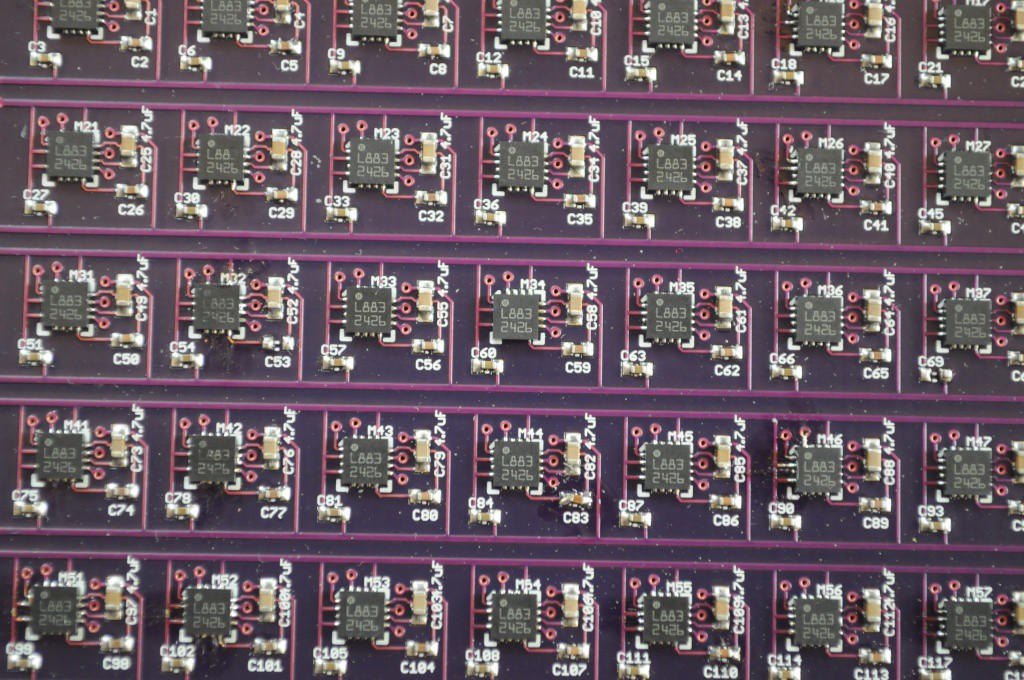
I admit that I don't fully appreciate what that will look like yet, because it's not entirely clear what the best configuration of code/gradient coils and such will look like -- but the idea of making a magnetic camera excited me enough a few months ago that I decided to make a quick sketch (in hardware), designed this experiment board and sent it off:
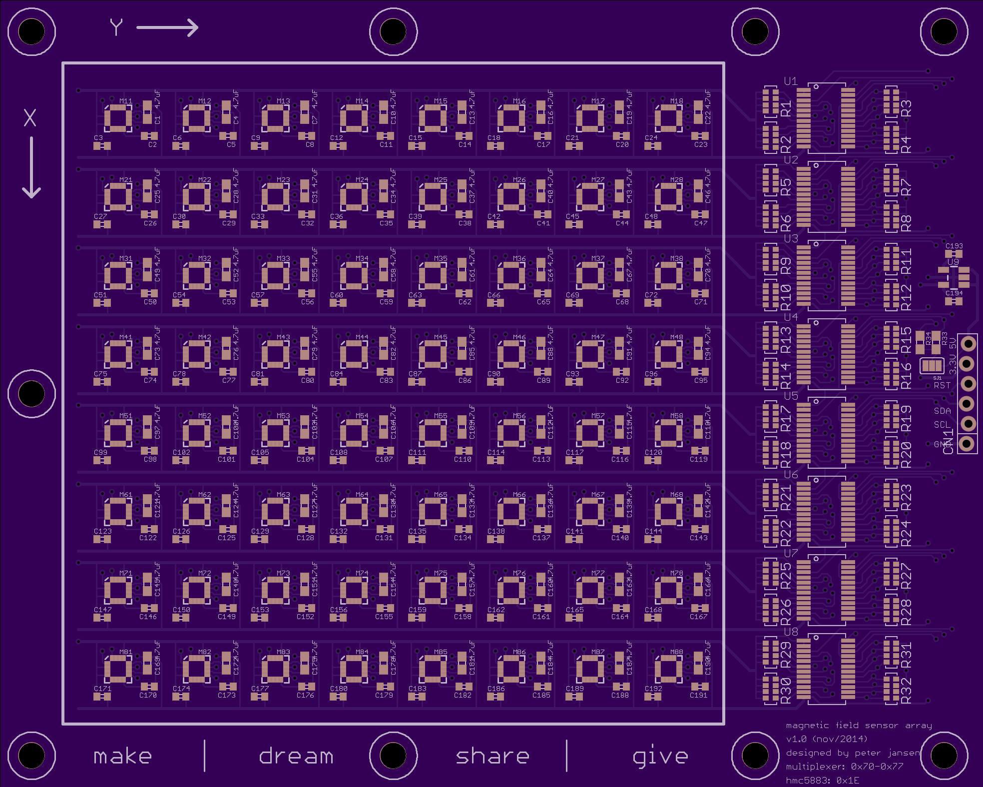
The board is an 8x8 array of the popular Honeywell HMC5883L 3-axis magnetometers that are very commonly used in the maker community (and for which a breakout board is available from Sparkfun). I chose the HMC5883L because they're very small (3x3mm), have the largest range I could find (+/-8000uT), and required a minimum of external components -- enough that I could get the packing efficiency to a 1cm grid on the camera board.
The HMC5883L communicates over I2C, and one of the issues with this is that all the sensors share the same address -- so I had to add in a bank of I2C multiplexers to be able to individually address each magnetometer. The benefit to this is that the entire array can be interfaced with using only 3.3V, GND, and two I2C pins, SDA/SCL.
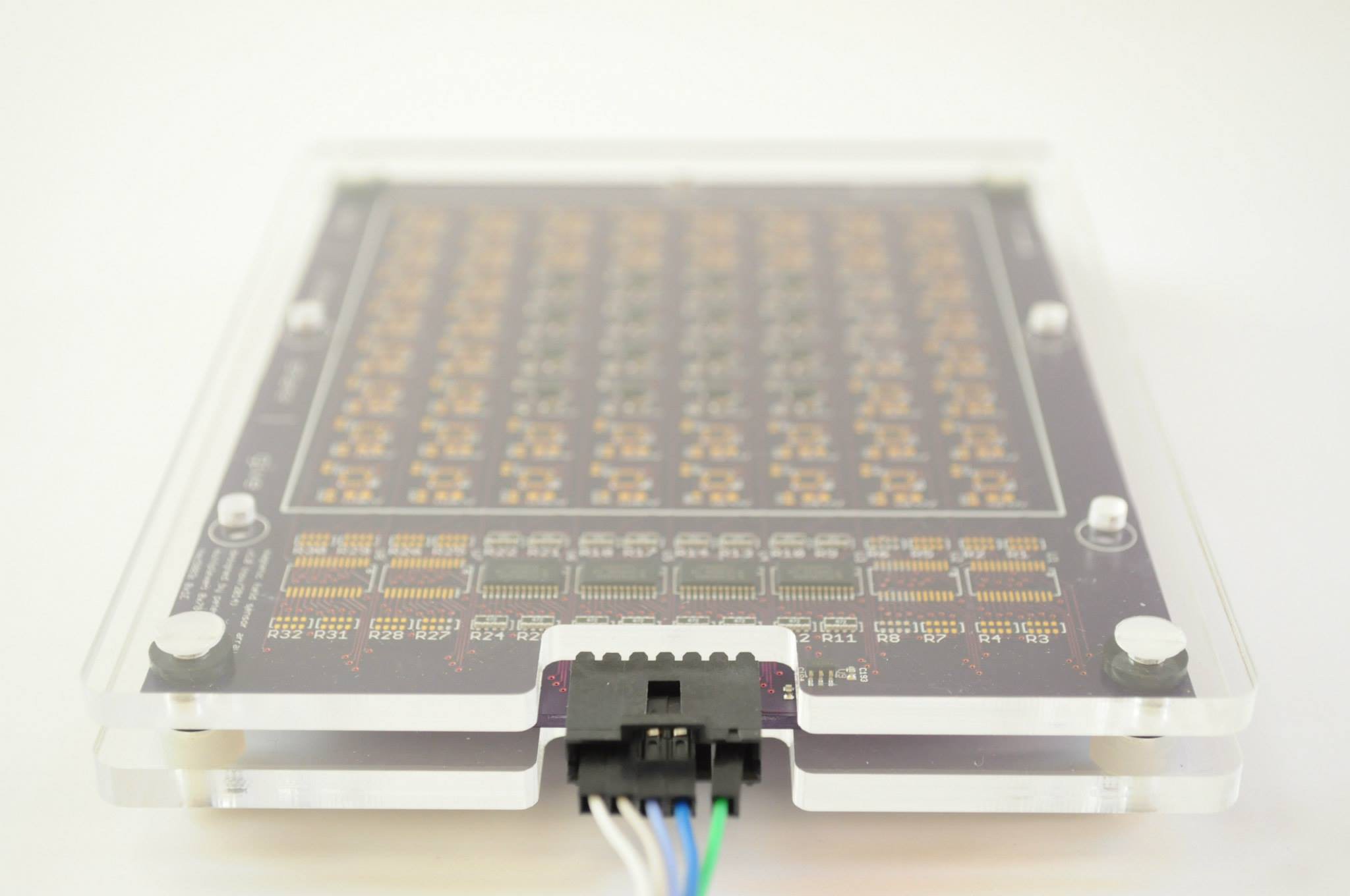
To initially test the design, I populated only the central 16 magnetometers in a 4x4 array, and made a plastic enclosure without any ferrous metals nearby.
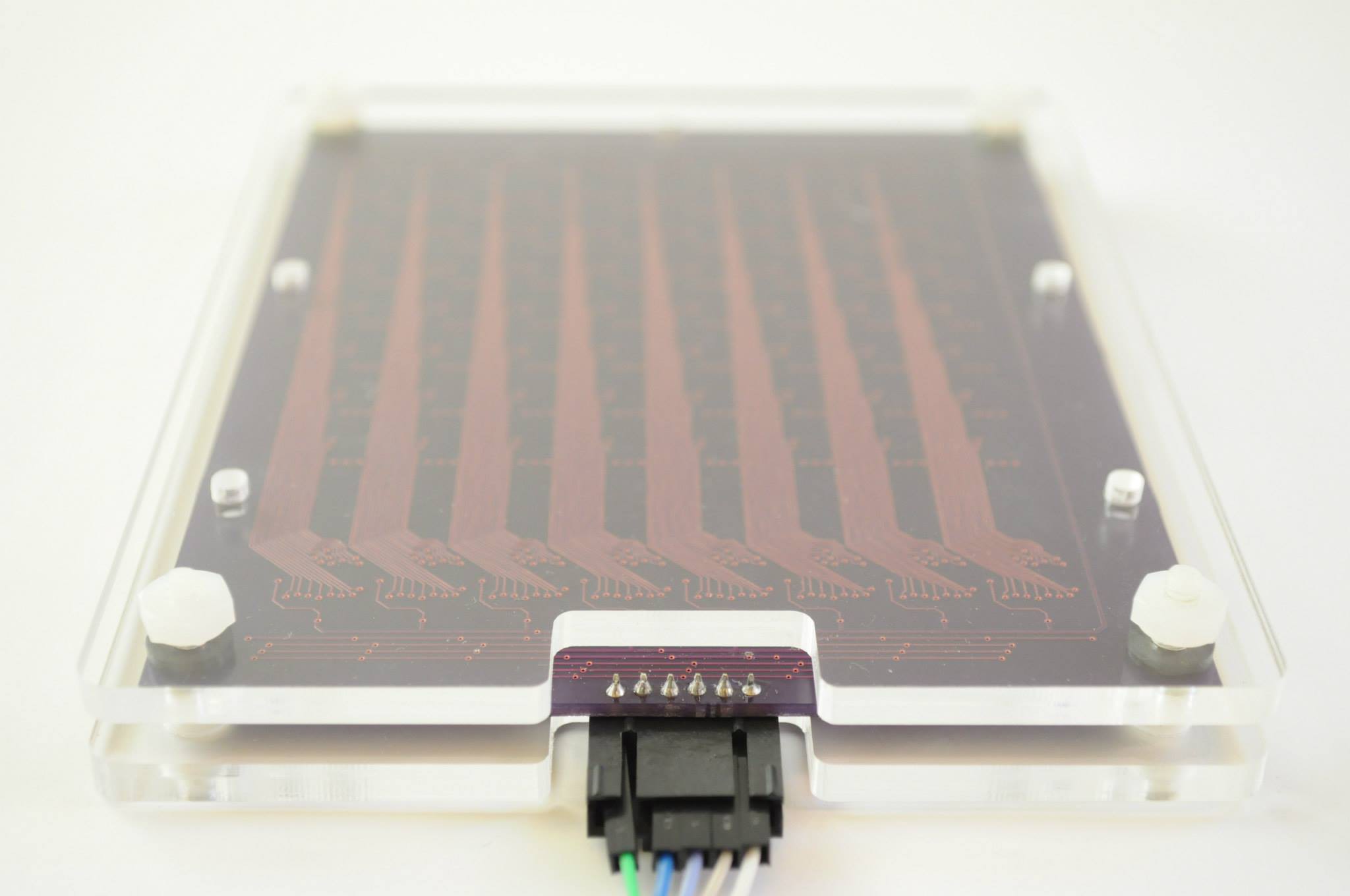
The board ended up working very well, and showed that the signals could be multiplexed in this fashion. A quick Arduino and Processing sketch showed that data was coming off, but a 1 cm grid is much too tiny to see interesting features -- it needs a mechanical scanning rig to scan the board in the x, y (+/-1cm), and z (+/- many cm) to generate images at a 1mm or lower resolution.
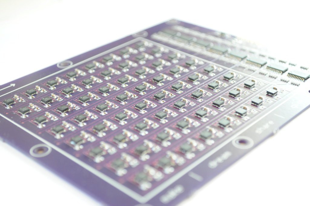
Unfortunately the story turns south here -- my hand stenciling abilities are not fantastic, and I don't have access to a proper stencil printer. The stencils that I use from OSHStencils are fantastic for the price, but they are quick to warn that Kapton stencils may not be ideal for very small pitched footprints (like the footprints for these magnetometers). I've found that the kapton stencils have worked well enough in the past even for these parts, but I'd never tried to align a stencil and uniformly deposit paste on a 10x14cm board covered with 200 tiny pitched magnetometers and 0402 capacitors. Still, against all warnings and inflated by my success with the 4x4 version, I gave it a try.
At first glance the stenciling looked okay, but on closer inspection many of the magnetometers had too much paste, and have very small bridges under them. I manually fixed about a dozen before admitting defeat, admiring the beautiful $200 coaster, and deciding that for an initial proof-of-concept, scanning a single magnetometer will likely be fine, it will just take 64 times as long. Once we figure out the final geometry, we can design a parallel detector, and ideally design it in such a way that we can make our mistakes cheaply when assembling it.
And so, onward.
About Us

I'm Peter Jansen, a Postdoctoral Research Fellow in artificial intelligence at the University of Arizona, where I work to try to teach computers how to learn and infer with concepts and language. I have an interdisciplinary background in cognitive artificial intelligence, computational neuroscience, astrophysics, optics, sensing, and signal processing. As the founder of the Open Source Science Tricorder project and a number of other open projects, I work to further science educational outreach and ground science education through sensing.
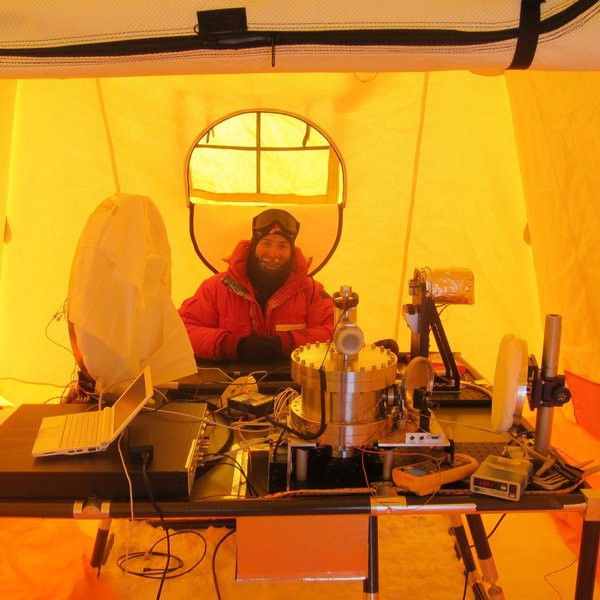
David Lesser, pictured here tinkering with a radio astronomy setup in a tent on a beautiful day at the south pole in Antartica, is an extremely talented and creative PhD candidate in radio astronomy at the University of Arizona. David has a great deal of expertise in designing (and using) electronics, radio equipment, and other such things that involve long wavelengths. He also knows his way around a machine shop, is much less frightened of an angle grinder than I am, and was once able to snag me some duct tape from a telescope machine shop when my radiator sprung a leak on top of Kitt Peak. Not that it's been held together by duct tape since then, or anything.
We both have a good set of common making skills, combined with a bunch of specific complementary expertise in radio, electronics, machining, fabrication, computational sensing, and simulation that make me at least 20% confident that we'll be able to put this together and make it work.
Thanks for reading!
Discussions
Become a Hackaday.io Member
Create an account to leave a comment. Already have an account? Log In.
Hello, I've read in one of the pages there that you're having memory issue (sorry I've lost the place) to store all the mesurements. I've worked on compressed sensing, it's a smart way to downsize the sample number without loosing data knowing some prior information. I've implemented it for an MRI on an internship. It may not revolutionize your stuff it's still nice to have. Send me an MP if you want to talk about it.
Are you sure? yes | no