Leonardo
-
First picture time
5 days ago • 0 commentsHi everyone,
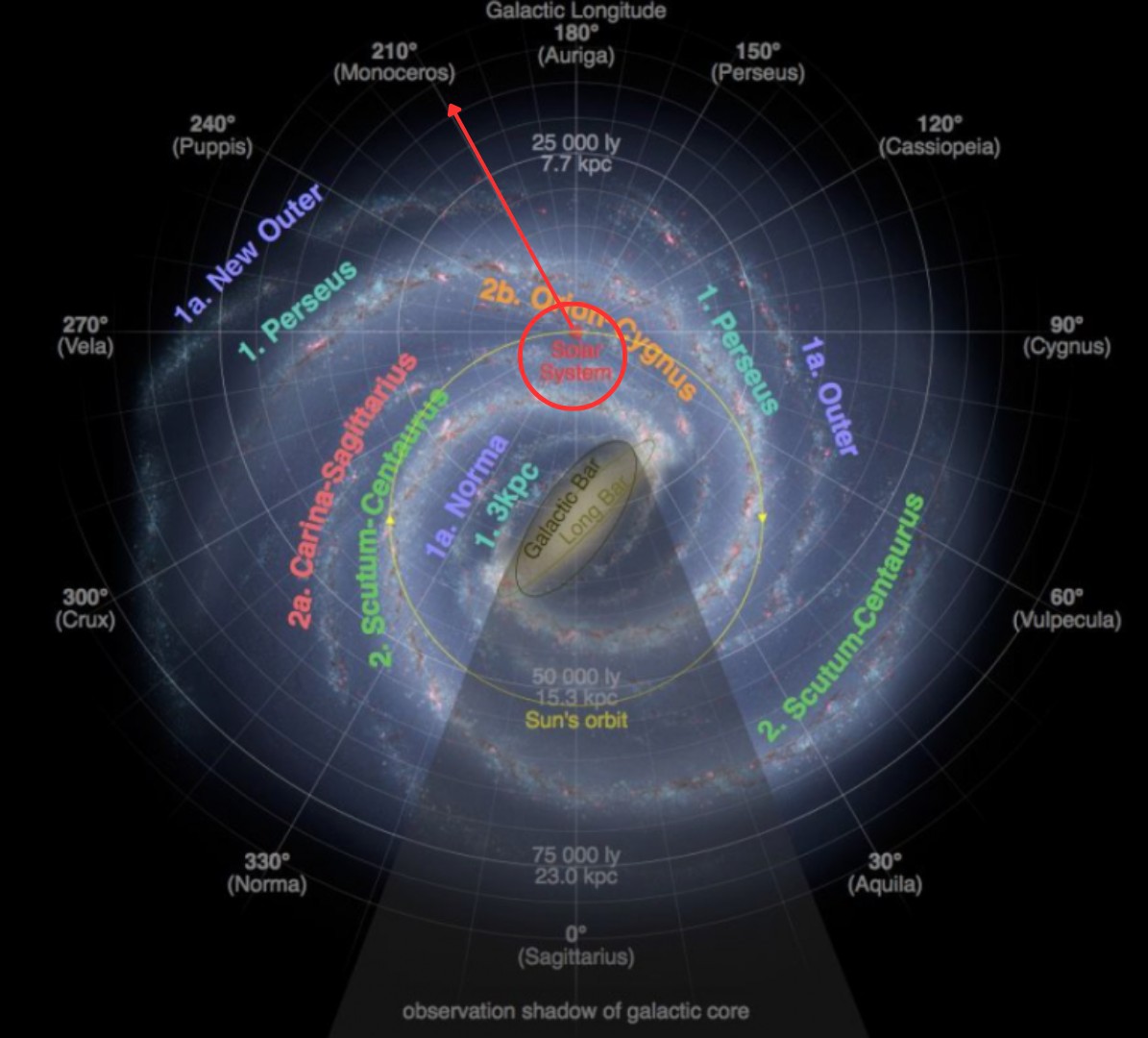
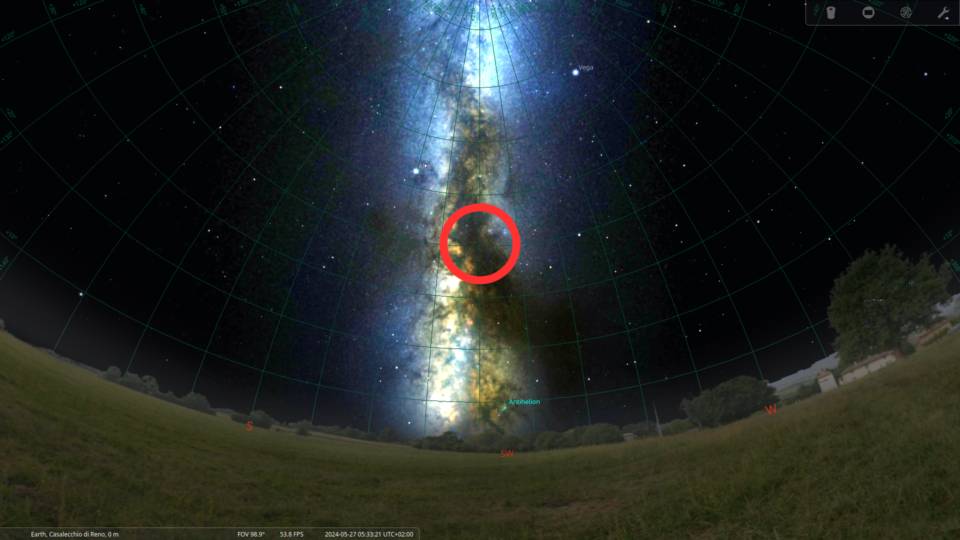
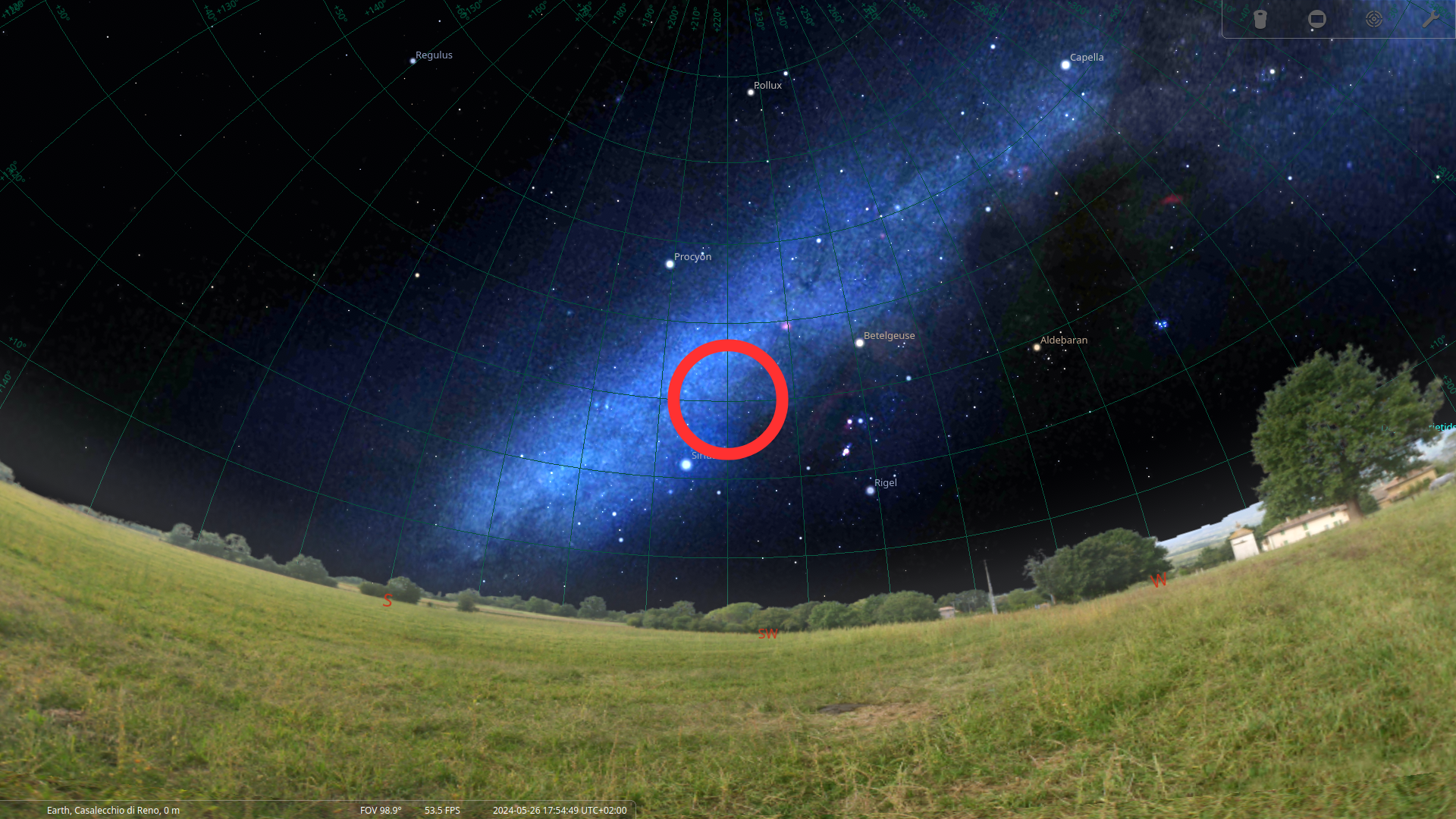
I just wanted to let you know that starting tomorrow I'll start collecting data for creating my first image of a part of the MIlky Way, the Perseus Arm.
Stay tuned.
-
24 hours experiment concluded!
05/27/2024 at 20:37 • 0 commentsHi everyone,
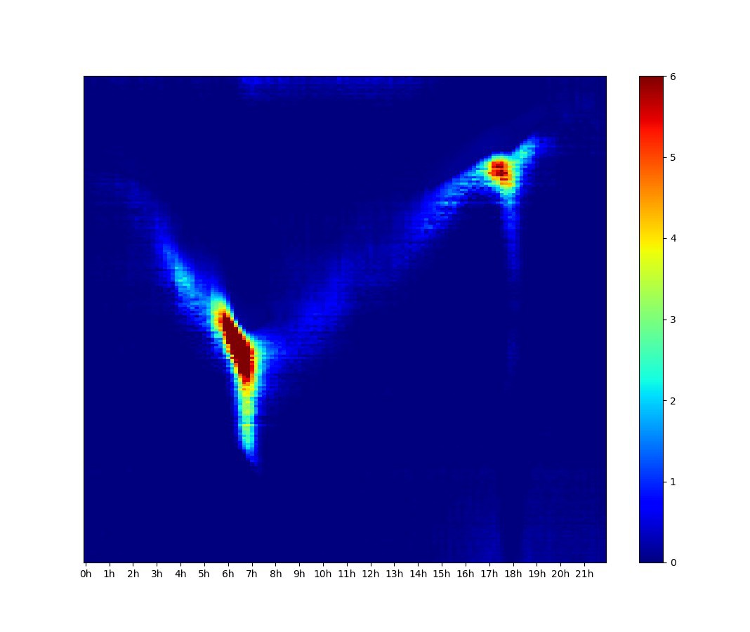
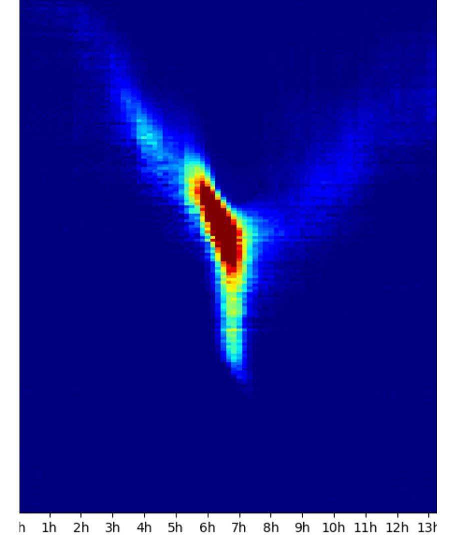
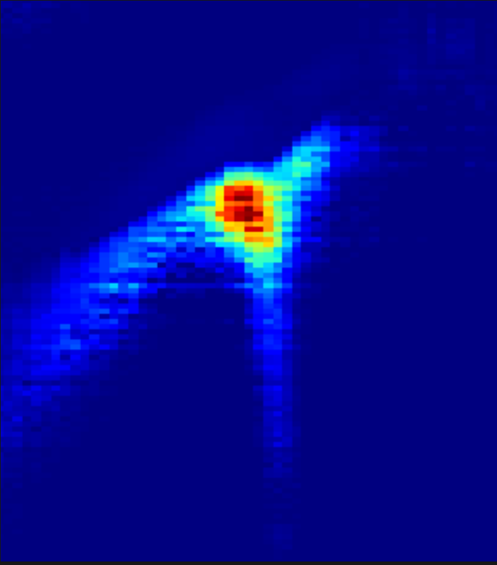
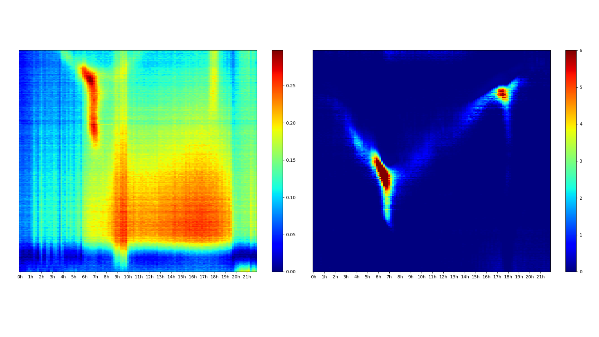
I just uploaded the report on the 24-hour experiment where my radiotelescope gathered data for an entire day, achieving really good results.
In the report, you can find insights on the new code I wrote for data analysis.
Go here to read the complete report.
EXPERIMENT GALLERY
![]()
![]()
![]()
![]()
![]()
![]()
![]()
-
Data gathering time
05/19/2024 at 20:45 • 0 commentsHi everyone,
just another quick update.
I've been experimenting with the radiotelescope and writing some interesting code to collect data autonomously over time.
I already have some really good results! I will share them as soon as I write the complete report.Additionally, I wrote an interesting algorithm to process the data and remove most noise; it works like a charm.
-
First results!
05/08/2024 at 13:47 • 0 commentsBig news today,
I just published the first results obtained with the radiotelescope.
Please read the article here, it's fascinating. -
Coding update (problems)
05/06/2024 at 17:01 • 0 commentsJust a quick update on the software side.
Although the code I published a few days ago is okay for displaying spectrum analysis results in other applications, my research and some testing have led me to conclude that that code is not useful in the field of radio astronomy. This is because it lacks some fundamental functions to obtain meaningful data during the pointing of astronomical objects, including:
- the ability to measure background noise and subtract it from subsequent measurements.
- the ability to integrate a series of measurements to obtain more averaged data with less interference/noise and, likewise, with amplified and visible signal peaks (what we want to see).
I am currently developing another code, which I will publish in the coming days. Stay tuned.
-
Antenna feed is ready
05/06/2024 at 16:54 • 0 commentsNews
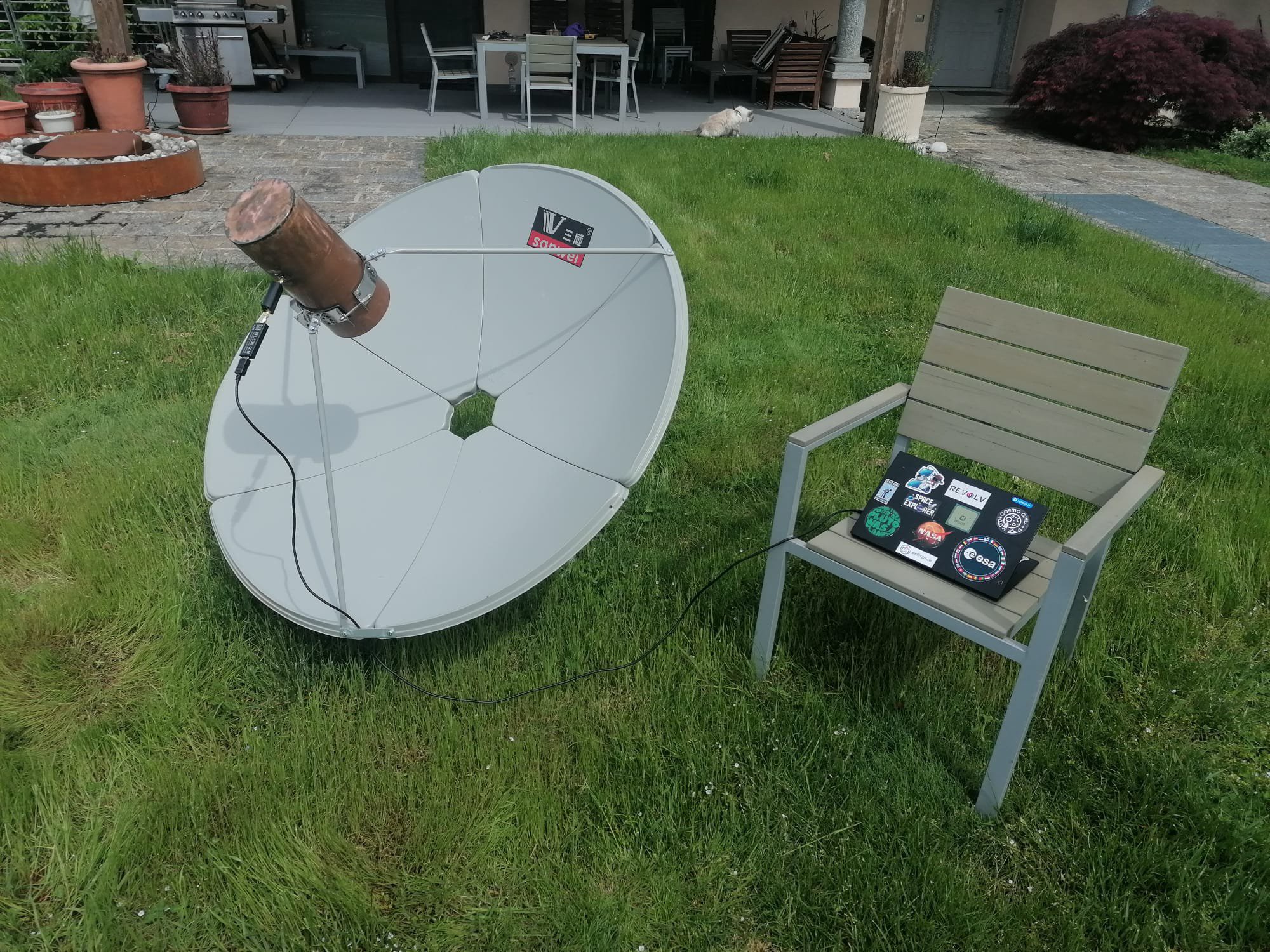
In the last few days, thanks to my father's help in soldering and assembling the device, the feed antenna for the parabolic dish is ready.
Design
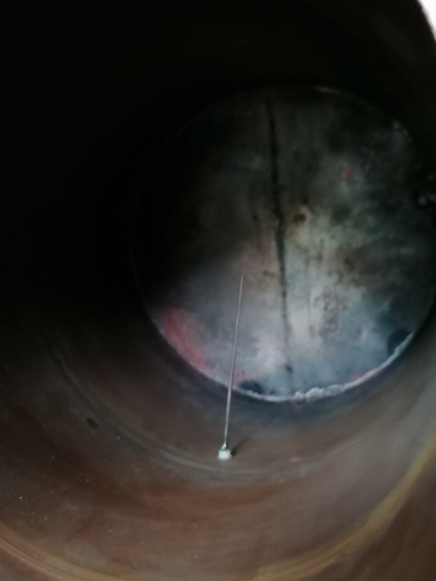
The feed antenna consists of a can-antenna made of a copper cylinder with a depth of 304mm and a diameter of 145mm. Additionally, at 101mm from the bottom of the cylinder, there is a straight copper wire with a length of 52.8mm (the actual antenna wire).
This design was created using this online tool (link here), in order to have a central frequency of 1420MHz, a lower cut-off frequency of 1212MHz, and an upper cut-off frequency of 1582MHz.
So, besides being centred on the frequency of the Hydrogen Line, it should also serve as an initial filter for the radiations we don't want to analyze.
Finally, an SMA connector was soldered to enable connection with a 50ohm coaxial cable to carry the signal from the feed antenna to the LNA and RTL-SDR.
Finally, in order to position this feed antenna above the parabola in the focal point area, an aluminium disk was fabricated to support the copper cylinder and to be connected to the 3 arms of the parabola typically used for satellite LNB connection (approximately 45cm above the bottom of the dish).
The aluminium ring allows adjusting the height at which the cylinder is suspended. My idea (to be verified) is that by lowering the feed antenna slightly below the focal point level, thus sacrificing some gain, the beam-width of the antenna becomes narrower, allowing me to aim more precisely at small astronomical objects.
Difficulties
- Soldering the copper cylinder.
- Soldering the SMA connector to the copper cylinder without damaging the connector.
Why a can-antenna?
This is a question I began asking myself right from the start and delved into further during the design of this feed antenna.
Firstly, the design solutions for a feed antenna typically involve horn antennas and patch antennas. Patch antennas are generally more challenging to fabricate at home without manufacturing errors significantly compromising performance. Horn antennas are also the most common type for these applications (just look at satellite LNB images), so my design would have followed that path.
Some online resources, particularly an intriguing video by Neptunium, showed how it was possible to use a cylinder instead of a horn for the feed of a parabolic antenna, possibly sacrificing some performance, but the compromise was entirely acceptable.
Gallery
![]()
![]()
![]()
![]()
![]()
![]()
( ! ) This setup is temporary, not the final design of the whole system.
-
Another coding night
04/30/2024 at 12:23 • 0 commentsJust a quick update.
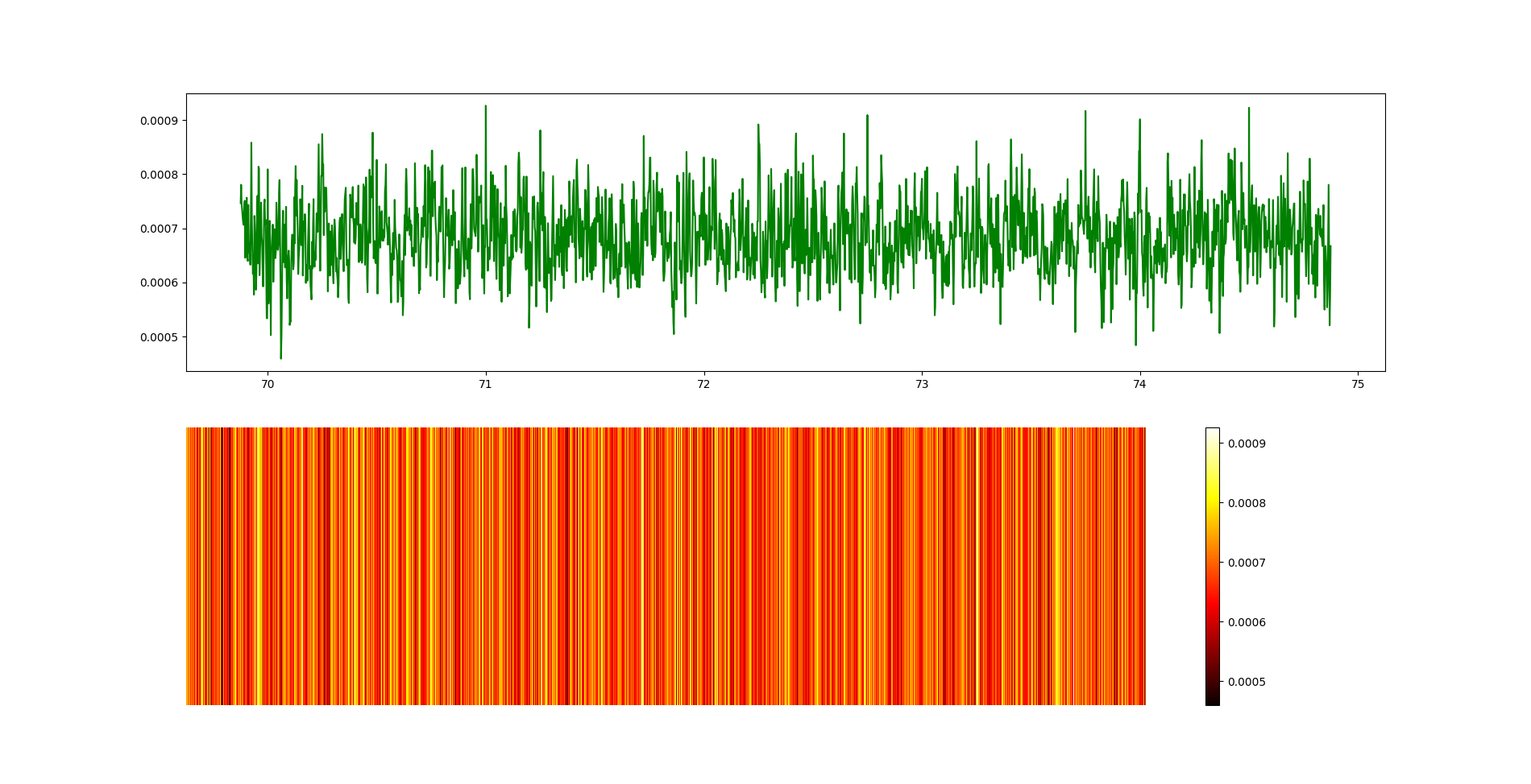
New Python code to display spectrum also with a heat-map.
from rtlsdr import RtlSdr
from matplotlib import mlab as mlab
import matplotlib.pyplot as plt
import os
from tkinter import *


# SETTINGS
GAIN = 4
SAMPLE_RATE = 2.4e6
F_CORRECTION = 60
DATA_RES = 128
try:
    sdr = RtlSdr()
except:
    print("Error: cannot initialize the SDR device")
    exit(0)

#ASK FOR FREQUENCIES
os.system("clear")
print("Insert initial frequency [MHz]: ", end="")
CENTER_FREQ = int(input())*1e6
print("Insert final frequency [MHz]: ", end="")
END_FREQ = int(input())*1e6

#CONFIGURATION
sdr.sample_rate = SAMPLE_RATE
sdr.center_freq = CENTER_FREQ
sdr.freq_correction = F_CORRECTION
sdr.gain = GAIN
garbage = sdr.read_samples(DATA_RES * 1024)
step = 2.5e5
half_step = step/2
center_f_arr = []
n = int((END_FREQ - CENTER_FREQ)/step)


def getdata():
    pow_arr = []
    freq_arr = []
    for k in range(0,n):
        sdr.center_freq = CENTER_FREQ + (step*k)
        center_f_arr.append((CENTER_FREQ + (step*k))/1e6) #save the central frequency for later
        samples = sdr.read_samples(DATA_RES * 1024)

        power, psd_freq = mlab.psd(samples, NFFT=1024, Fs=sdr.sample_rate/1e6)
        psd_freq = psd_freq + sdr.center_freq/1e6

        for i in range(0, len(psd_freq)):
            if psd_freq[i] < (sdr.center_freq+half_step)/1e6 and psd_freq[i] > (sdr.center_freq-half_step)/1e6:
                freq_arr.append(psd_freq[i])
                pow_arr.append(power[i])

        if(len(freq_arr) > 536870000):
            print("Fatal error: trying to store too much data")
            exit(0)


    i = 0
    for e in freq_arr:
        if e in center_f_arr:
            pow_arr[i] = pow_arr[i-1]
            pow_arr[i+1] = pow_arr[i+2]
            pow_arr[i-1] = pow_arr[i-2]
        i=i+1
    return freq_arr,pow_arr


#ask for data
freq_arr,pow_arr = getdata()

#create 2d map
mappa = [[0 for x in range(len(pow_arr))] for y in range(len(pow_arr))]
for i in range(0, len(pow_arr)):
    for j in range(0, len(pow_arr)):
        mappa[i][j] = pow_arr[j]


f, axarr = plt.subplots(2)
axarr[0].plot(freq_arr, pow_arr, color="green")
c = axarr[1].imshow(mappa, cmap='hot', interpolation='nearest',origin ='lower', aspect='auto')
axarr[1].axis("off")
f.colorbar(c)
plt.show()
Output plot:
![]()
-
Coding night
04/26/2024 at 21:25 • 0 commentsJust a quick update here.
I've been messing around with the RTL-SDR Python Library to get some readings from the SDR dongle.
In the end, I managed to make the first version of code that takes two frequencies as inputs, and after some time shows me the spectrum results gathered between those two frequencies.
The code has been developed to remove the typical "central frequency spike" caused by the 0MHz reading and to be as flat as possible between multiple readings, which is necessary because one reading only has 1MHz of bandwidth.
from rtlsdr import RtlSdr
from matplotlib import mlab as mlab
import matplotlib.pyplot as plt
import os

try:
	sdr = RtlSdr()
except:
	print("Error: cannot initialize the SDR device")
	exit(0)

os.system("clear")
print("Insert initial frequency [MHz]: ", end="")
CENTER_FREQ = int(input())*1e6

print("Insert final frequency [MHz]: ", end="")
END_FREQ = int(input())*1e6

GAIN = 4
SAMPLE_RATE = 2.4e6
F_CORRECTION = 60
DATA_RES = 128

pow_arr = []
freq_arr = []

# configure device
sdr.sample_rate = SAMPLE_RATE
sdr.center_freq = CENTER_FREQ
sdr.freq_correction = F_CORRECTION
sdr.gain = GAIN
garbage = sdr.read_samples(DATA_RES * 1024)

step = 2.5e5
half_step = step/2
center_f_arr = []
n = int((END_FREQ - CENTER_FREQ)/step)

#init loading bar
bar = "["
for i in range(1,n+1):
	bar = bar + " "
bar = bar + "]"

#main loop
for k in range(0,n):
	sdr.center_freq = CENTER_FREQ + (step*k)
	center_f_arr.append((CENTER_FREQ + (step*k))/1e6) #save the central frequency for later
	samples = sdr.read_samples(DATA_RES * 1024)

	power, psd_freq = mlab.psd(samples, NFFT=1024, Fs=sdr.sample_rate/1e6)
	psd_freq = psd_freq + sdr.center_freq/1e6

	for i in range(0, len(psd_freq)):
		if psd_freq[i] < (sdr.center_freq+half_step)/1e6 and psd_freq[i] > (sdr.center_freq-half_step)/1e6:
			freq_arr.append(psd_freq[i])
			pow_arr.append(power[i])

	os.system("clear")
	string_list = list(bar)
	string_list[k+1] = "="
	bar = "".join(string_list)
	print(bar)
	print("Frequency: ", end="")
	print(psd_freq[i])

	if(len(freq_arr) > 536870000):
		print("Fatal error: trying to store to much data")
		exit(0)


i = 0
for e in freq_arr:
	if e in center_f_arr:
		pow_arr[i] = pow_arr[i-1]
		pow_arr[i+1] = pow_arr[i+2]
		pow_arr[i-1] = pow_arr[i-2]
	i=i+1

print("\n")
print(len(freq_arr))
print("\n")
plt.plot(freq_arr, pow_arr)
plt.plot(END_FREQ/1e6, 0.005)  #noise visual filter
plt.show()
It's just a very alpha version of the code and needs a bit more work, but for now and for some early testing, it's enough.
-
New RF components
04/26/2024 at 11:16 • 0 commentsNews
I wanted to give you a quick update on the radio telescope development.I've just received some new RF components that I'll be installing over the next few days.
These comprehend:
• Various SMA cables and connectors
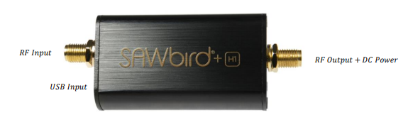
• Noolec SawBird+ H1 LNA
• RTL-SDR Blog V3 (should be here tomorrow)Also, I started designing the Feed Antenna of the dish. Basically, a can-antenna
designed to have a lower cut-off frequency of 1212MHz and an upper cut-off
frequency of 1582MHz.
[link to the design tool]Noolec SawBird+ H1 LNA
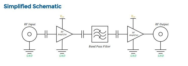
Nooelec SAWbird+ H1 is a SAW Filter & Ultra-Low Noise Amplifier (LNA) Module for
Hydrogen Line (21cm) applications with a center frequency of 1420MHz.
Some key features of this LNA are:
• +40dB of RF gain at 1420MHz
• 0.8dB noise figure at 1420MHz
• +3.3V-5V single supply![]()
![]()
If you don’t know what an LNA is you should check out this link. I will upload a more detailed document in the “Insights” section of the repository on GitHub where I’ll talk about LNAs.
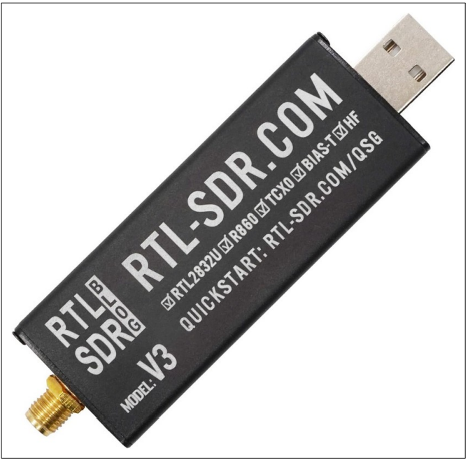
[link to this LNA datasheet]RTL-SDR Blog V3
![]()
The RTL-SDR Blog V3 is a key component in our project setup. It's essentially a software-defined radio (SDR) dongle built around the Realtek RTL2832U chipset.Widely adopted by hobbyists and professionals, it serves a range of purposes, from radio monitoring to spectrum analysis and amateur radio activities.
Its affordability and compatibility with open-source software make it an ideal choice for my project's needs. I will post more insights on this device as the project evolves.
My idea is to write Python code to read data from this dongle to enable more interesting data processing.
-
Assembling the parabolic antenna
04/26/2024 at 11:02 • 0 commentsNews
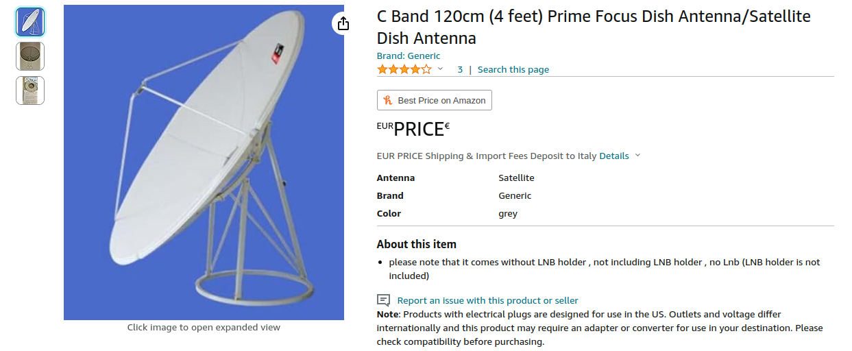
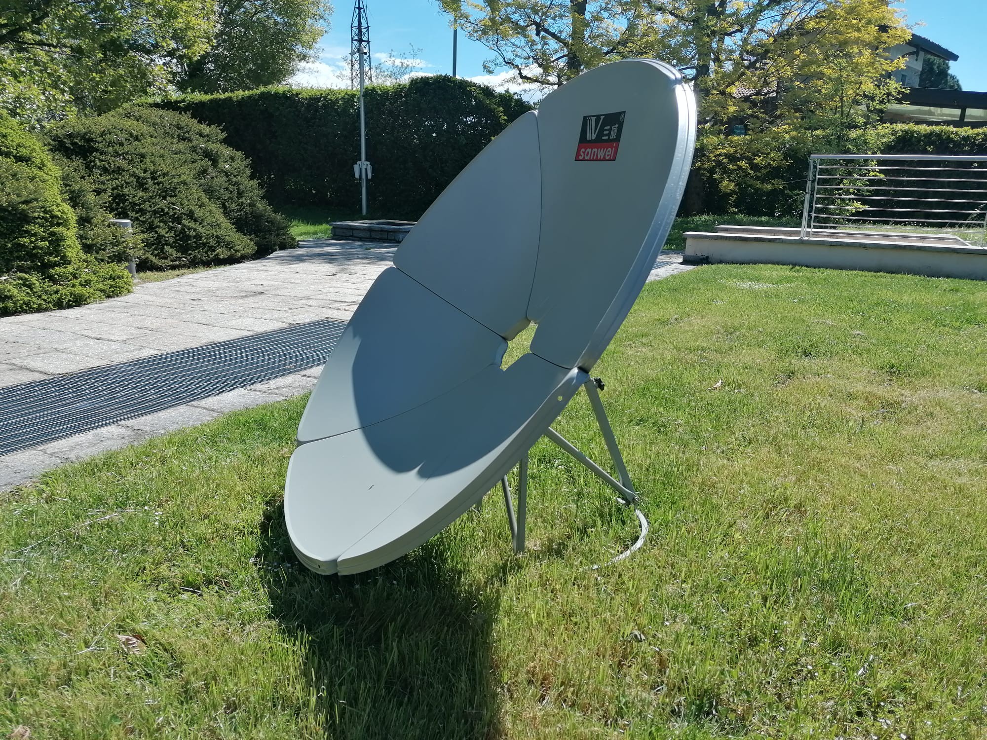
In the past few days, I've had the opportunity to order online and then assemble
the parabolic antenna for the radio telescope. It has a diameter of 1.2m, a
depth of about 20cm, and therefore, a focal point height of approximately 45cm.
The antenna was sold with a simple aluminium stand on which to mount the dish and
which allows for adjusting the antenna's pointing angle.
The only thing is that it's not sold together with its metal LNB Holder ring. No
big deal though, because it's a piece I would have built anyway in order to
accommodate my custom receiver (Feed Antenna) which will then receive the
amplified radiation from the dish.![]()
Why a parabolic antenna?
Unlike other types of directional antennas, such as Yagi antennas, these allow for the amplification of a much wider signal band.
This will enable the radio telescope to study other astronomical frequencies in the future, as well as the Hydrogen Line. Moreover, this type of antenna guarantees a high amplification factor while still maintaining relatively small dimensions.
This one, in particular, is a primefocus parabolic antenna, meaning that the focal point of the antenna (where the receiver will be positioned) is at the central position.
More commonly seen are offset parabolic antennas, where the focal point and LNB are at the bottom of the antenna. However, these are more difficult to point towards a particular target.![]()