Let's see how the cables measure influence the range of the reflectometer. How do the noise filtering mode and methods for determining the unknown propagation coefficient affect the measurement accuracy?

KEY FACTORS FOR CABLES

The reflectometer's detection range depends on the cross-section of the cable cores, the overall quality of the cable, as well as on the way the reflectometer is connected to the cable being tested.
The larger the cross-section of the cable cores, the less attenuation the electrical pulse supplied by the reflectometer to this cable undergoes and the longer the distance it covers.
Old or defective cables may have reduced insulation resistance or increased attenuation. This significantly reduces the ability of the cable cores to conduct electrical signals and, as a result, reduces the maximum distance.
The connection of the reflectometer to the cable must be done so that a pulse with the maximum possible amount of energy is emitted from the reflectometer to the cable.

NOISE FILTERING

I want to eliminate the noise in more detail, as it is on any cable. Many reflectometers have a digital noise filtering mode that obliterates the noise from 50 Hz to 1 GHz. This mode is designed primarily for lineworkers dealing with cables near sources of strong electromagnetic interference (for example, railway contact networks, power lines, or antenna poles). The operator can select a filter type with the required characteristics for each test to ensure the acceptable quality of the resulting reflectogram.
Suppose an unexpected random voltage value appears in the line during the measurement. In that case, the noise-filtering mode gets turned on automatically.
A multi-level and multifunctional filtering system allows one to check antennas and cellular nodes with some received signal interference.

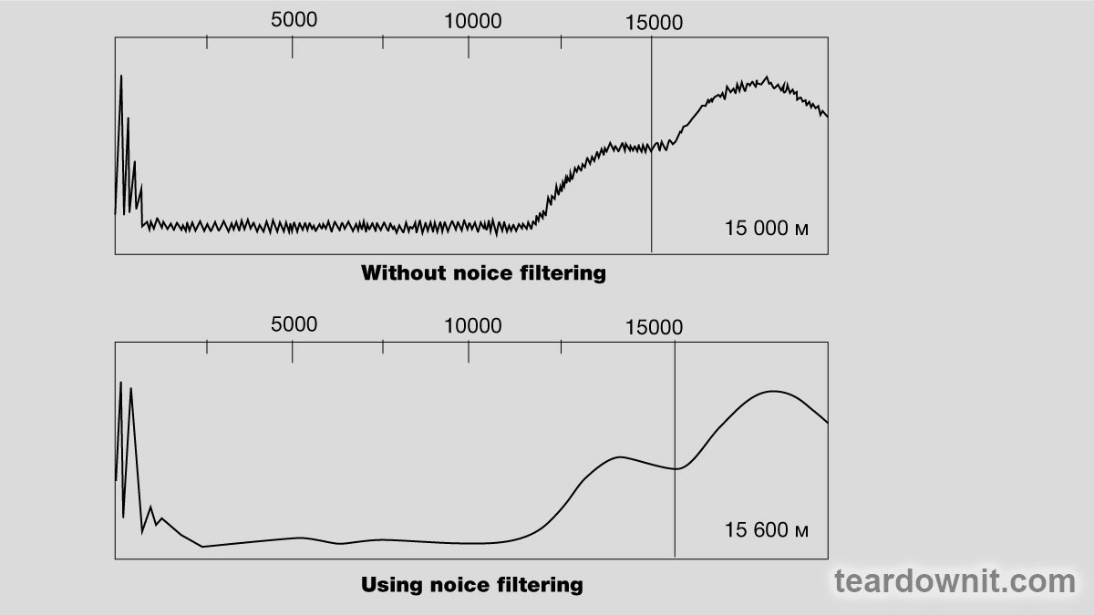
In some cases, the noise-filtering subsystem may slow down the OTDR operation to such an extent that the display becomes unusable. A good example is filtering the noise the power supply induces (60 Hz). One period of alternating current with a frequency of 60 Hz is 16.7 ms. Therefore, it also takes 16.7 ms to generate one point on the reflectometer display. It will take no less than 5.12 seconds to refresh all the 256 image pixels on the display. One way to compensate for this delay is to store the denoised reflectogram. Writing data to the device memory will take some time, but subsequent operations will be as fast as if the filter were turned off.

The "averaging" mode, often provided by the manufacturer to eliminate interference at maximum gain, is no exception. This mode also decreases the refresh rate of the display. Four times less noise means the screen is refreshed sixteen times slower. When the image refresh speed is reduced significantly, it becomes difficult to work with the display, so this mode should be used only when necessary.
One more thing to mention: cables for digital data transmission should be tested using short pulses with a duration of 2, 10, or, in extreme cases, 100 ns. They do not affect nearby pairs under load, so the data transmission devices' error detection system will not flag them as such.

PROPAGATION COEFFICIENT AND METHODS FOR ITS DETERMINATION

As already mentioned, the reflectometer determines the distance to the abnormal spot based on the signal propagation speed in the cable and the time it takes to reach the point in question and return. In most cases, speed is expressed as a unitless coefficient, the ratio of the signal propagation speed in a given cable to the speed of light. It is an empirically determined value. Reflectometers from different manufacturers require one to set the wave propagation speed, called the Velocity of Propagation (VOP) or Velocity Factor (VF). Typically, this parameter is expressed as a fraction of the speed of light and can have a value from 0.3 to 1. A cable with a VOP value of 0.66 allows an electrical signal to be transmitted at 66% of the speed of light. Some manufacturers express this parameter in terms of actual speed, and then it can range from 45 to 150 m/ms.
The choice of the VOP (VF) parameter significantly impacts the accuracy of any measurement made. Therefore, to obtain the most correct results possible, it is necessary to learn the methods for determining the propagation factor for each specific cable.

VOP DETERMINATION METHODS UNDER DIFFERENT CONDITIONS

Suppose the pulse propagation coefficient for the cable is unknown. In that case, an experiment can either calculate or determine it.

1. The insulating material's dielectric constant (ε) is a known value.

VOP=1/√(ε),

where ε is the relative dielectric constant for a given cable. For example, for polyethylene, ε = 2.25. Therefore, VOP = 1/√2.25 = 0.667.

2. For the first experiment, one needs a short cable of the same type as the tested cable.
Connect the reflectometer to the cable section and adjust it so that the pulse reflected from the end of the section is clearly visible on the display. Move the cursor to the beginning of the pulse and start changing the VOP coefficient until the measured distance to the end of the cable is equal to its actual length (mind the length of the leads).
The longer the cable, the more accurate the obtained VOP value will be.

3. A similar experiment occurs when the cable length is known, and it has a non-defective pair.
Connect the reflectometer to the pair and adjust VOP until you get the cable length you already know on the screen. Again, account for the probing leads.
Suppose this technique is applied to thick multi-pair cables. In that case, ensuring that the reference and tested pairs belong to the same cable layer is necessary. The length of a pair of outer layers significantly exceeds the length of a pair of inner ones.

4. If the cable length is known, but there is no suitable pair for comparison, then it is necessary to have access to the cable from both sides.

Roughly pick a VOP value and determine the approximate distance (L1) to the fault on side A. Using the same VOP value, determine the approximate distance (L2) to the fault on side B.

The exact distance to the damage can be calculated with L1 and L2.

From side A, according to the formula:
(L1/(L1 + L2)) x L, where L is the known cable length.
From side B, according to the formula:
(L2/(L1 + L2)) x L, where L is the known cable length.