 Hugh Brown (Saint Aardvark the Carpeted)
A short video showing how I've managed to get consistent impacts by building a cardboard Da Vinci hammer can be found here:
0%
0%
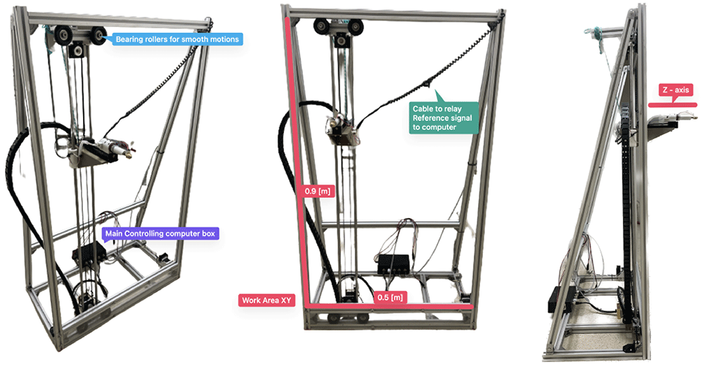
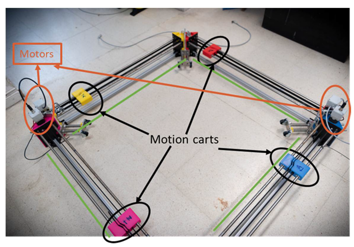
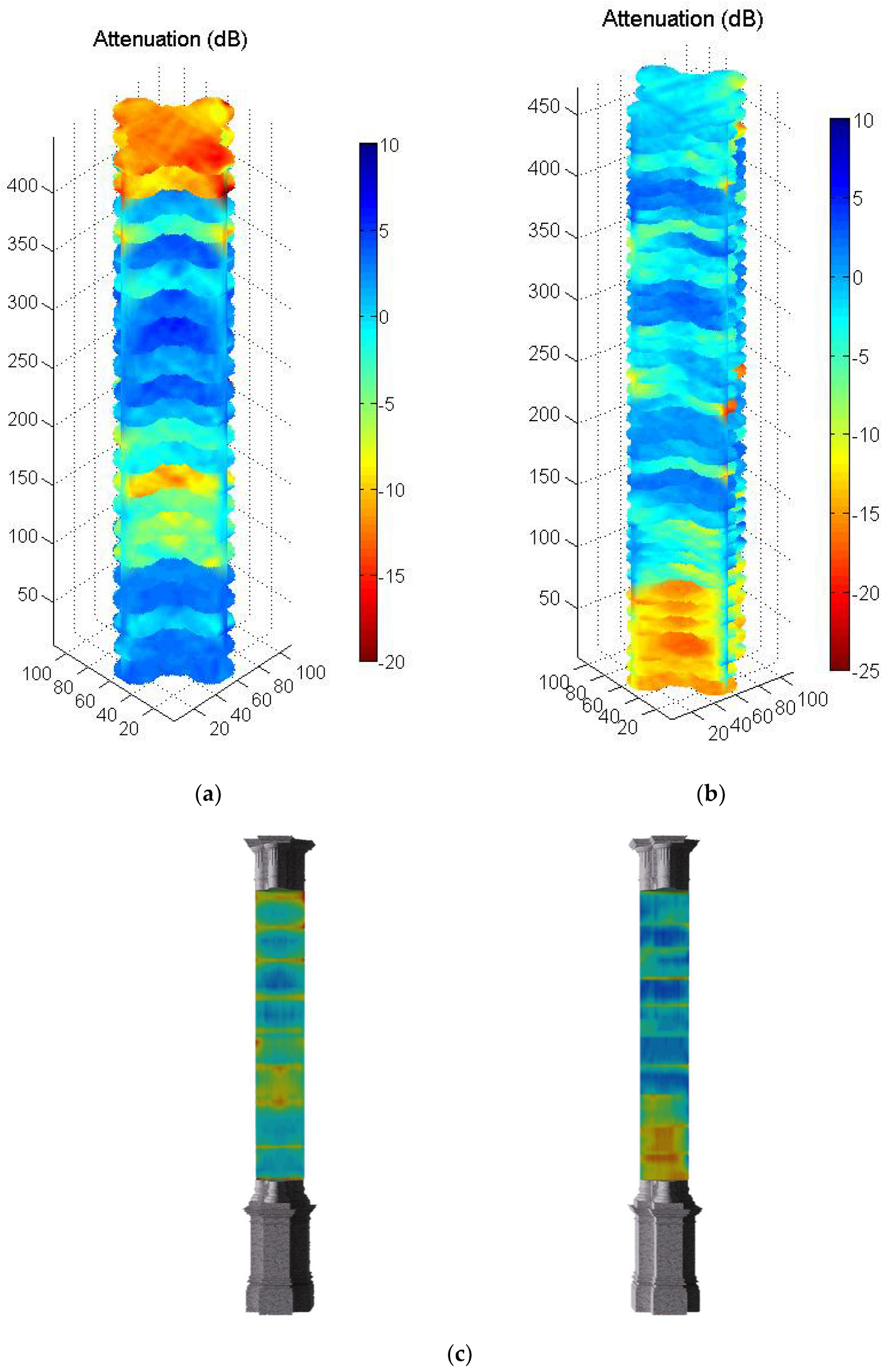
Exploring the internals of trees with sound
Time-of-flight, tomography and more
Become a Hackaday.io member
Already have an account? Log in.
Just one more thing
To make the experience fit your profile, pick a username and tell us what interests you.
Pick an awesome username
hackaday.io/
Your profile's URL: hackaday.io/username. Max 25 alphanumeric characters.
Pick a few interests
Projects that share your interests
People that share your interests
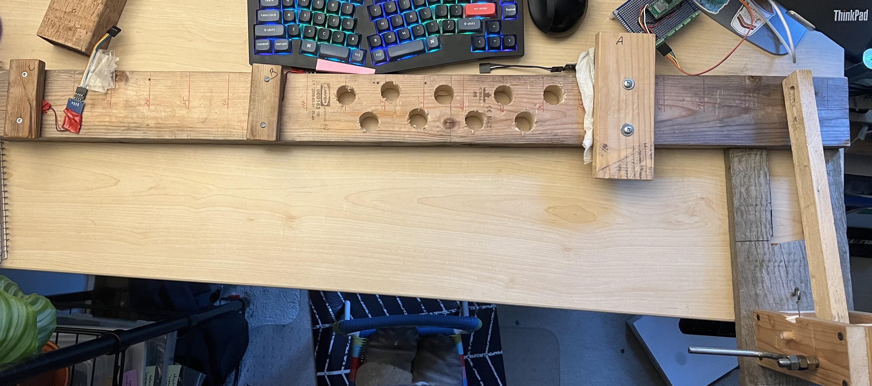
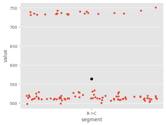
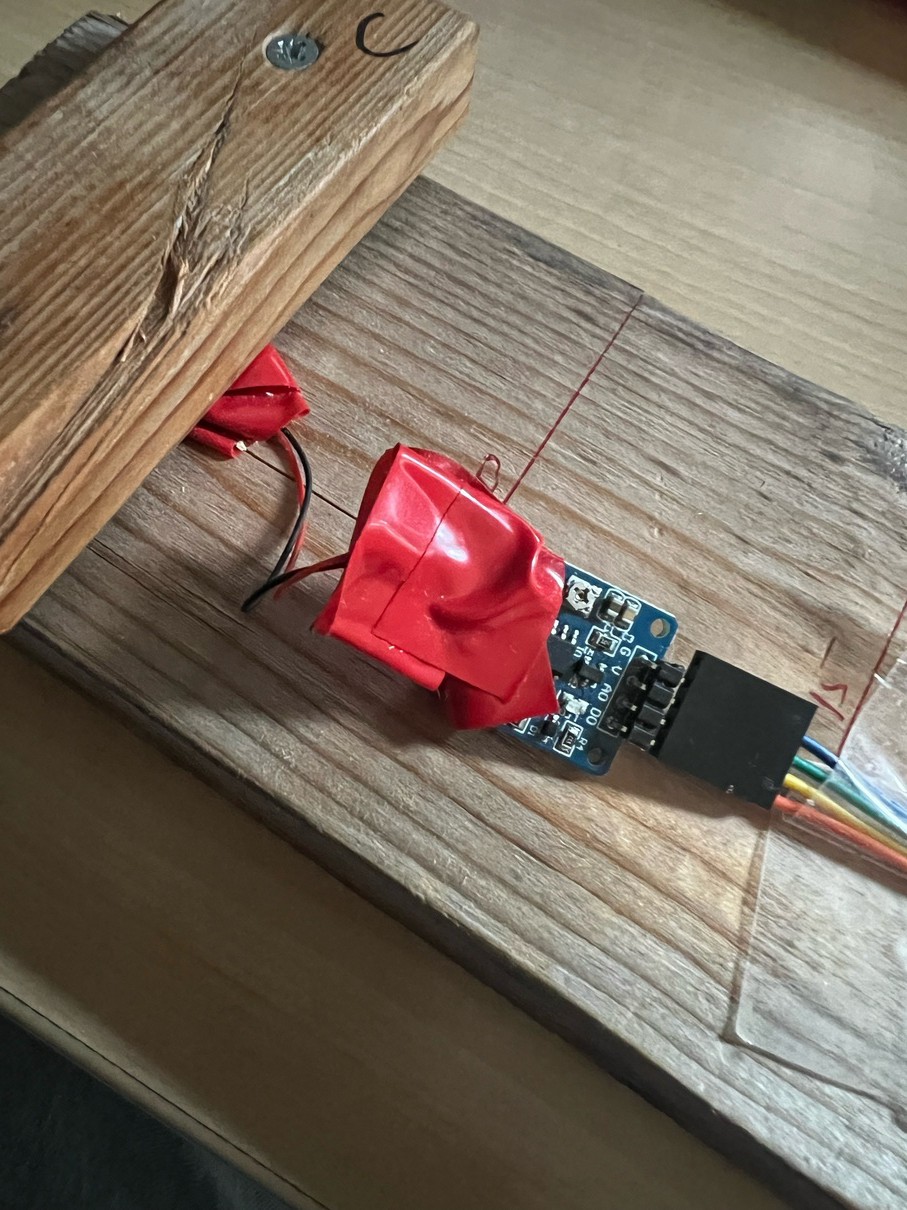
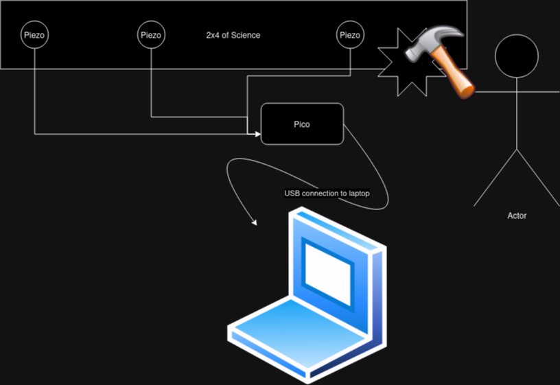
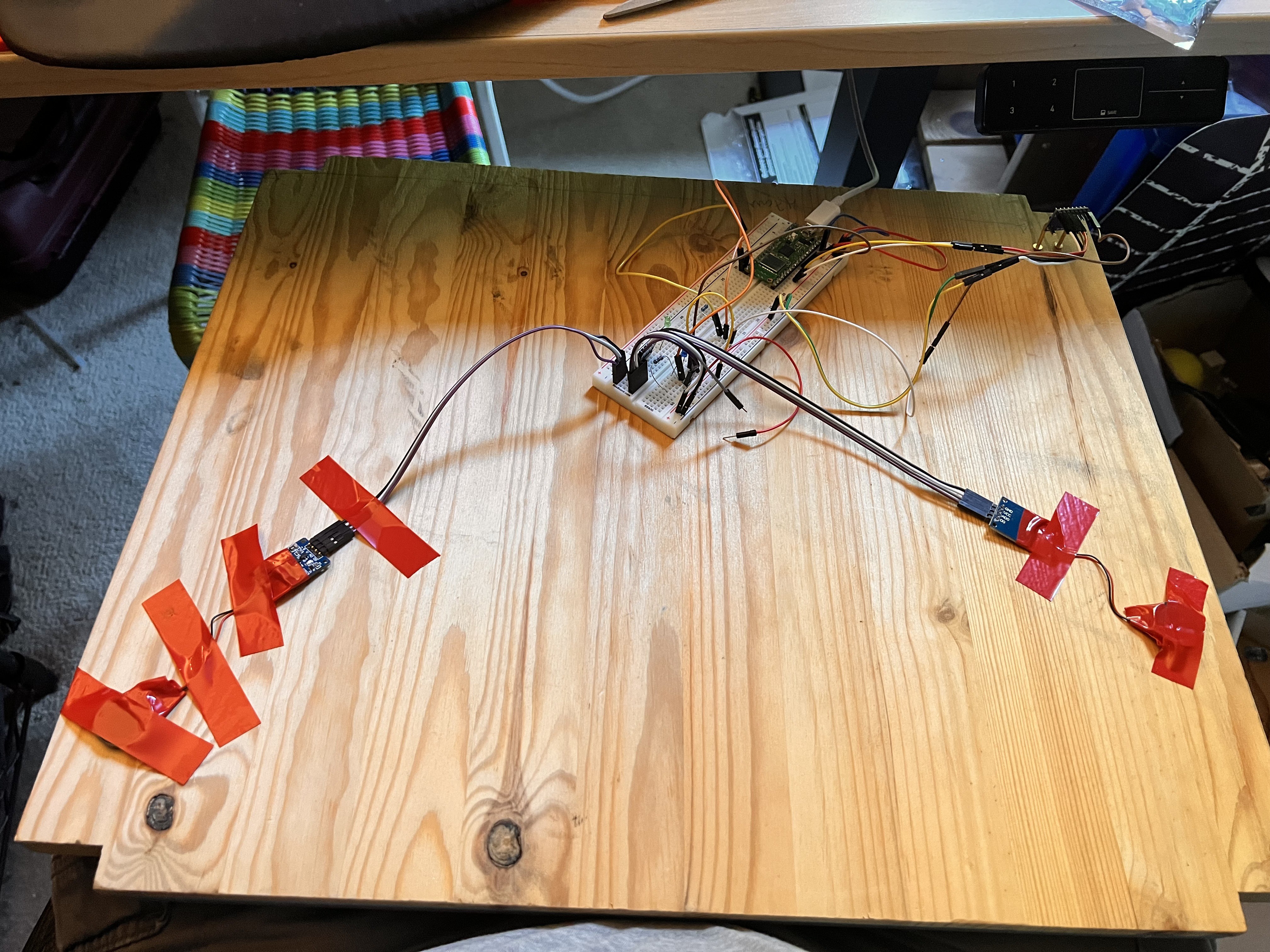
 I copy-paste that into my editor, run awk to massage it into CSV form, then paste it into LibreOffice. I move the sensors to B and C and re-do the process, then again with sensors A and C. That gives me time of flight for each segment. I then export the spread to another CSV file (now with headers & columns for each segment), and add that to
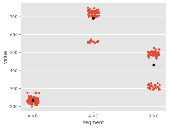


 peter jansen
 Johannes
 kwan3217