Table of Contents
2.1.Statements of Aims, Objectives, and Motivation
2.3.Advantages of Hexapod over Wheeled Vehicles
2.4.Disadvantages of Hexapod over Wheeled Vehicles
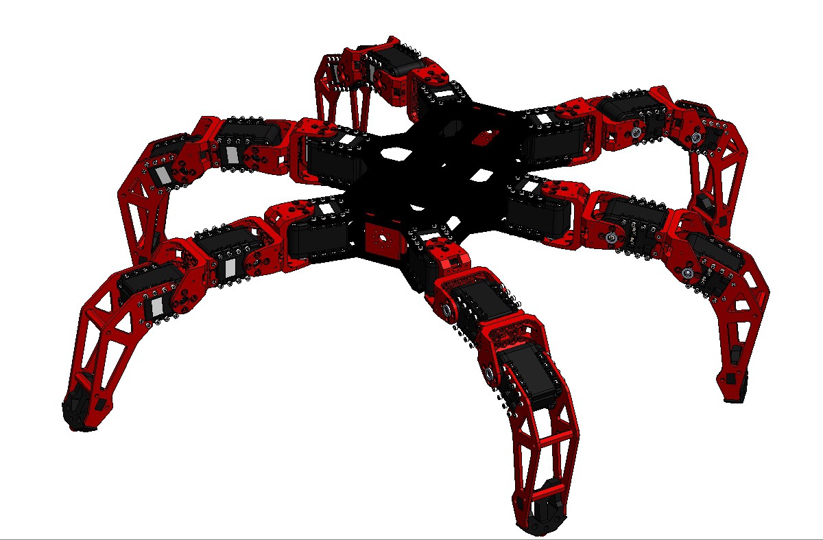
3.Fundamentals of Hexapod Robot
3.1.1.Swing and Stance phases of a Hexapod
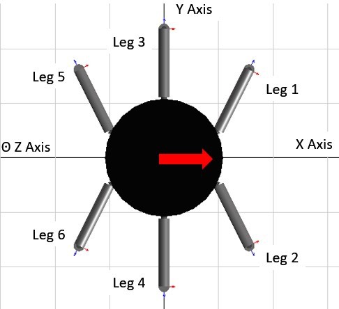
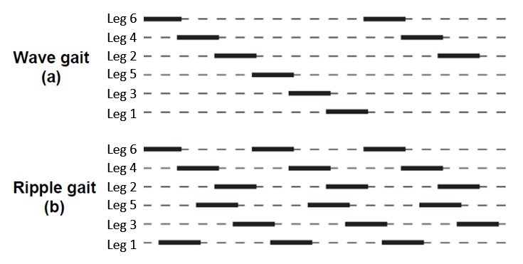
3.1.2.Tripod Gait, Wave Gait, Ripple Gait
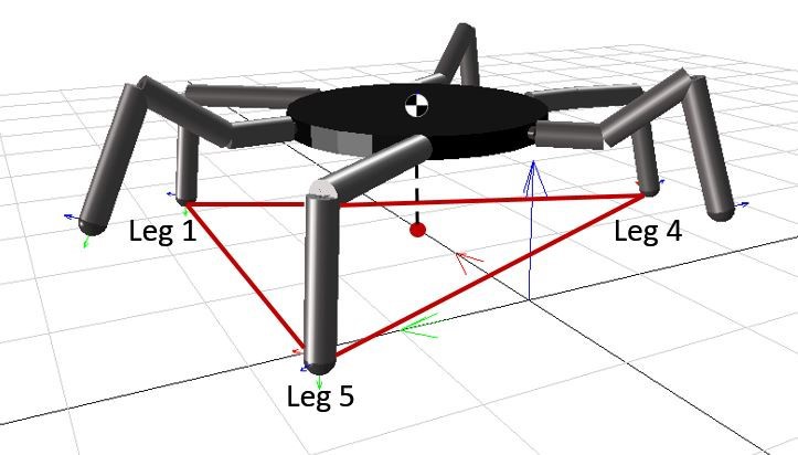
3.2.Stability of Hexapod Robots
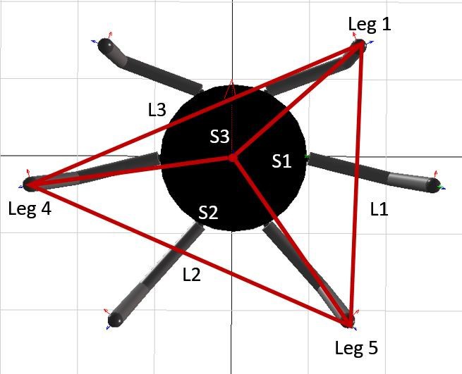
3.3.Kinematics of Hexapod Robot
3.4.1.Dynamic Model of the Leg Mechanism
4.Hierarchical Control Architecture
4.3.2.Stability Detection and Recovery
8.Appendix
8.1.Additional Visuals
8.2.Additional Equations
8.3.MATLAB Code


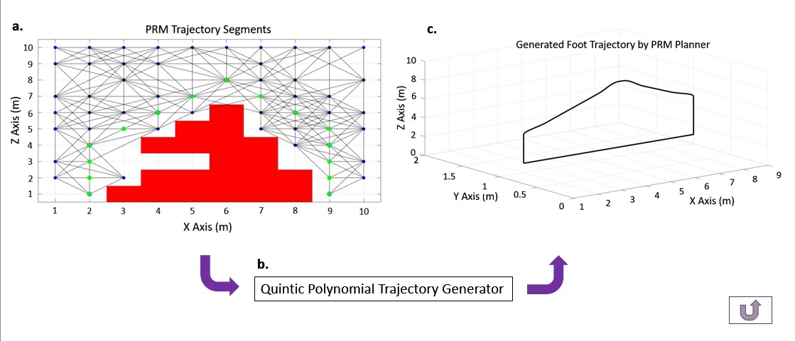
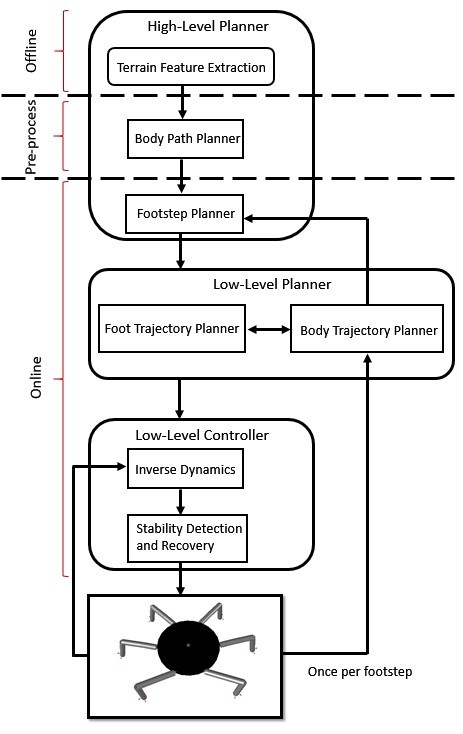
 Figure 4.2-a Uneven terrain and the 2D representation of terrain, adapted from [15]
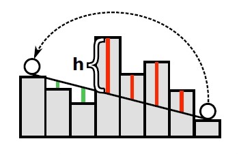 Figure 4.3 Collision map of a foot trajectory over an obstacle, adapted from [28]
 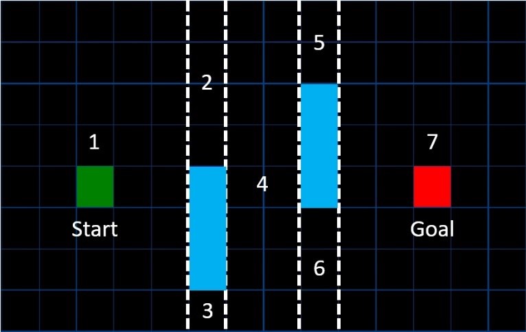 Figure 4.4 Occupancy Grid Representation
 Figure 4.5 Adjacency Map of the Occupancy Grid.
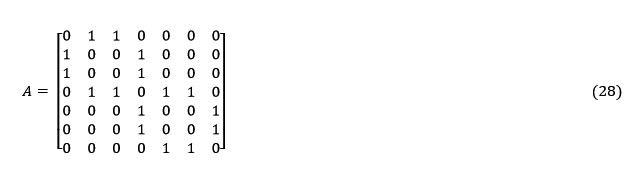 A* (star) path planning algorithm determines the cost of the 8 surrounding nodes by using Equation 28,
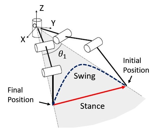

 ssla-couk
 Cirmall
 Nyeli Kratz
 ensafatef
This is great! Are you planning on posting the source code for this project?