Phased array pulse design

Continuous wave or CW

First a couple of links to some background explanations:

Link: Radar tutorial on CW

Link: Radar tutorial on range resolution

CW pulse

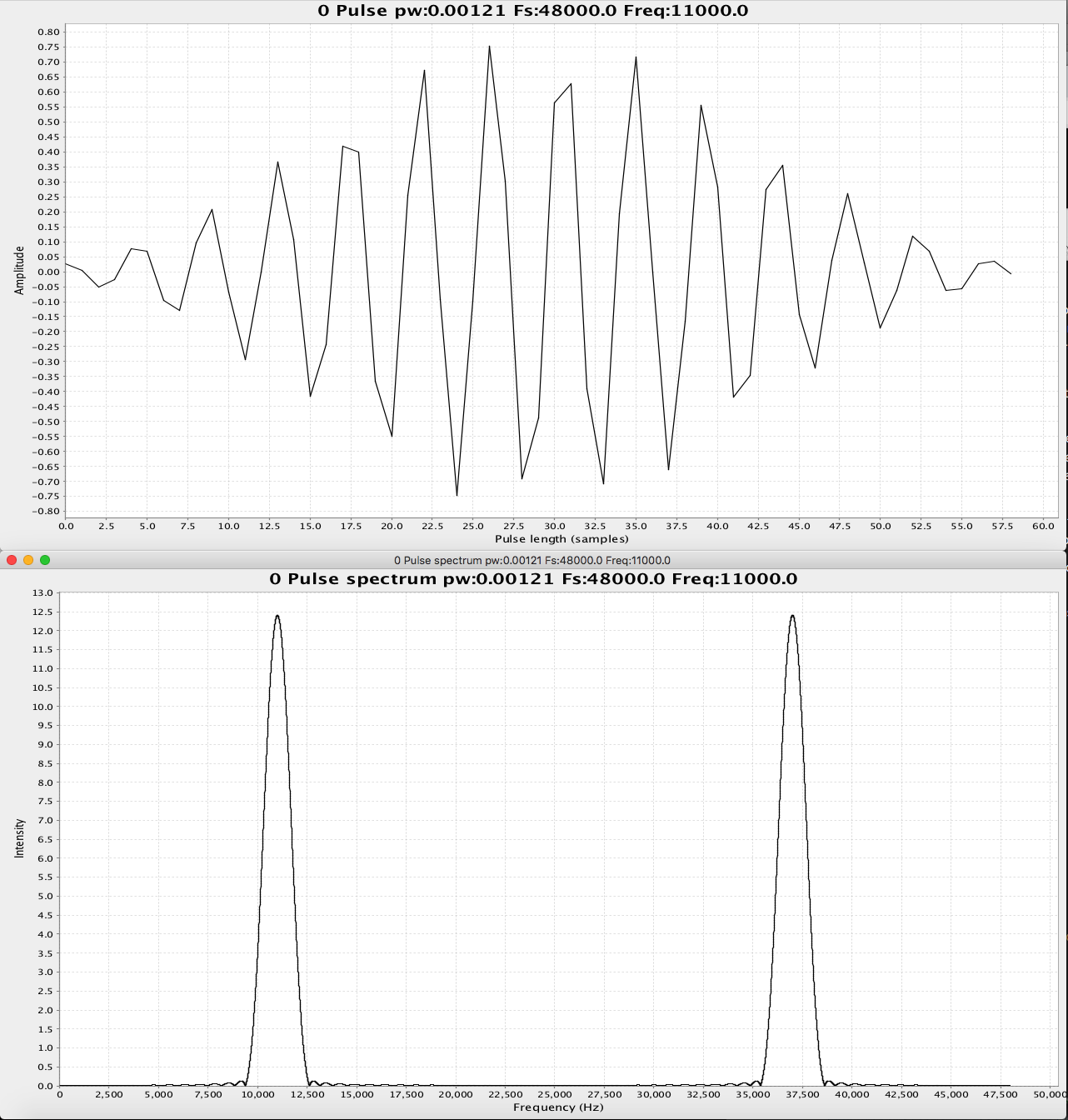
CW pulse consist of a constant frequency and a duration (pulse length).

Range resolution is:

where c is the speed of sound (in air 330m/s).

So to get a range resolution of 2cm, we need a pulse length of 121us.

If sampling frequency is 48000Hz, the CW pulse is approx. 6 samples long.

Pulse length vs. bandwidth

There is an inverse relationship between pulse length and bandwidth of the transmitted signal. 

The short pulse, have a wide bandwidth.

Likewise, if pulse is 10 times longer we get

Narrow bandwidth on a longer pulse.

With a narrow bandwidth, will be able to process the signal to only listen to those specific frequencies and filter out noise. Further, sending long pulses require less energy to transmit to reach the same distance. Drawback is that range resolution worse (10x to be exact).

Spectrum has a main lope, the signal we want to process, but it also has a lot of side lopes, which is unwanted signals.

We can manage the side lopes using window functions. There are a lot of different windows function designs, with different properties. Boxcar (rectangular), Hamming, Kaiser, Chebychev to name a few. The latter are pretty good at suppressing side lopes, but the cost is a wider main lope.

Some perspective, a wide main lope will make our objects in the beam formed image wider. Objects will look wider than they are, so a wide main lope is not what we want.

Again, we want narrow beams, good range resolution so we can identify the objects in the image.

An example with a Kaiser window function applied to the transmitted (long) pulse

Side lopes are almost gone, but the main lope is wider.

CW pulses are easy to understand, require less post-processing to generate great looking images. But total range might suffer, as short pulses requires more energy.

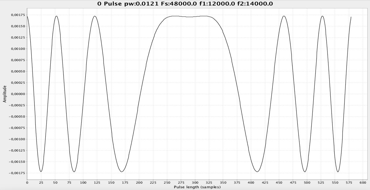
Intrapulse modulation (or FM)

If we, instead of transmitting short pulses, transmit longer pulses with a frequency change, a sweep from frequencies F1 to F2, built in, AND post process the signal with range compression (using a match filter), the properties of range resolution is defined as:

where BW is the bandwidth of the transmitted signal. Notice that the range resolution is no longer dependant on pulse length (in theory at least). The larger the BW is, the better range resolution we get.

Example: range resolution of an FM transmitted signal where f1=12000Hz and f2=14000Hz is approx 8.25cm. 

Example of FM pulse, linear chirp.

Link: Radar tutorial on Intrapulse Modulation

Pulse compression

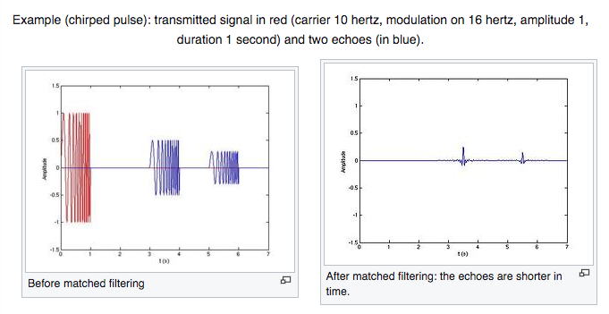
Pulse compression is a filter that matches the transmitted pulse with the received data. It filters out data that is not correlated with the pulse, hence increase S/N significantly.

(source wikipedia: https://en.wikipedia.org/wiki/Pulse_compression)

Red pulse is transmitted and when pulse hits objects, the are reflected, the blue echos are returned. When applying the match filter, the impulse response is shortened to the short "blips", seen to the right (hence compression of the pulse).

I real life sonars, data is echos from the objects and surroundings and the compression filter aka match filter, removed every thing else but the matching pulse.

A sonar ping under water, will contain background noise from the surroundings, maybe engine noise from a ship or similar. This is effectively removed so only data echoed from the transmitted pulse remains.

Match filter can be processed in frequency-domain

where MD is the resulting data after match filtering, RD is the raw received data and pulse is the transmitted pulse.

In my project, I use the frequency-domain implementation, since its running in CUDA 

Above is basically just a FIR filter. You could use the same implementation to remove...

Phased array signal processing

Link: IQ data for dummies

Link: Generating Complex Baseband and Analytic Bandpass Signals

Link: I and Q Components in Communications Signals and Single Sideband

IQ (In-phase and Quadrature)

There are a lot of literature that explains the dark-magic around IQ signals, but in essence, together they form a complex number, which can be represented as a real and imaginary value - or magnitude and phase.

I and Q amplitude form a combined amplitude and a phase.

When two waves (complex IQ) are mixed, the phase difference between to two waves determine if resulting wave will undergo constructive or destructive interference.

Given two microphones that records a sound from some angle, the same sound is recorded by both microphones, but with a time delay. The time delay corresponds to the angle from where the sound originated or a difference in phase between the two signals.

Time delay for element j (tde)

where angle is the direction that we want to listen (steering the beam), pde(j) is the phase for element j, and c is the speed of sound

Phase delay for element j (pde) in array:

where ne is the number of elements in the array, d is the element spacing

Sample delay for element j. Note that "center" channel is the ne/2'th element. 

Sampling the data from the elements (channels)

When sampling data from the array's elements, we sample real values. The phase is missing from the sampling.

To generate the phase in order for us to generate the IQ data, we need to run the Hilbert transform

where real is the sample data per channel and iq (in timedomain)

Combining all the channels with IQ data, we get a NxM matrix of IQ data, where N (rows) is the number of samples per channel and M (col) is the number of channels.

Beam forming using FFT

Beam forming the data i.e. transforming the data from time domain frequency domain or from channels to beams is simple:

where IQ is in frequency domain and FFT is a 1D transform in the channel direction

Now each col in the matrix represents the frequency data in angle direction.

Angles in the beam formed data:

where i is the i'th beam, c is the speed of sound, ne is the number of elements, d is the element spacing, f is the frequency.

Note that the angle now become dependant of the frequency of the signal. Listening to multifrequency signals like whale song, changes (calculated) angle when whales sing. FFT's are probably not the best way to detect direction when frequency varies

Example:

If we want to calculate the angle for a f=200kHz, where ne=256, d=0.02m for the beam i=100, the angle is -0.51 degrees. Changing the frequency to 220kHz, the angle is -0.47deg. A small change, if we do a chirp.

Using f=2kHz, the angle is -64deg and for f=3kHz, the angle is -37deg. The frequency sweep is impossible to beam form for lower frequencies with larger bandwidth.

Beam forming using CZT transform

Chirp-Z transform or zoom-FFT is a variant of the FFT. It consist of 2x forward FFT and 1x Inverse FFT, so its requires 3x computations. The advantage is that the CZT allows us to specify the angles in the transform, basically letting us zoom into a pre-defined angle-space. 

One of the biggest advantages is that the angle calculations are independent of the frequency. Angle space is the same, regardless of the frequency, which is what we want.

Further, we can specify the angles in the angle space we want to use, where as the FFT is pre-set to a specific angle space.

where a1 and a2 are the zoom angles, ne is the number of elements. Notice that angle space is only defined by the zoom angles and number of elements.

Clearly, CZT is the preferred beam former, if FFT's are to be used.

Further, the open angle is worth to revisit.

Open angle specify the outer limits of the a1 and a2, we make sure that we do not conflict with the grating lopes of the beam radiation pattern. This will cause "mirror" effects in the final image.

Example:...

Phased array tests

Beamforming tests

First test is to send a CW signal and record the response on the 16 channels. The result is beamformed and visualized as a polar-image, where angle-range is plotted. Range is in meters, angels is in deg.

Total range: 30m

Swath is pre-set to the open-angle, as decribed above. Right is the color-scale. Resulting image is built up of 5-pings. Images are stacked. Stacking process removes some of the specke-noise or background noice and amplifies the objects. 

The brighter lines are actual objects that reflect the ping. Distance is measured by counting samples and convert to meters. Looking closely at the image, we can see that the objects fade above 15m out. The room I am testing in, is much smaller so everything above 1.5m-2.5m out is multipath or sound reflected off walls and furniture. 

Similar distance measurement, like the SR04 is designed to detect objects within the swath and closer than 5m. Above image shows objects more than 15m away, plus where they are.

The CW pulse is short, 100us long, which require more power to transmit in order to get further away. 

One solution is to use a different pulse, FM (frequency modulated) where frequency sweeps. Using this in combination with a matchfilter, we can use longer pulses, 0.5ms-3ms, so less power is needed. Result should be that we can detect objects further way that the 15m.

Total range is 50m. 

Notice the object just above 35m and -7deg. This is not visible using the CW pulse.

On purpose, I have not interpolated the beams in the above images. This is to highlight how wide the beams actually are and how large the objects are.  The 16 channels have been oversampled into 128 beams, which explains why the objects witch seem larger than the beam-width from the beamforming. 

The oversampling trick is especially interesting when we apply movement to the sonar, similar to what mobile phones are doing with super-resolution. The use multiple images and align them to get an even higher resolution image.

Back to phased array project...