The goal
The goal of this project is to try and have a simple machine vision system, trained to do one thing, do it as good as possible with the available resources and do it fast, really fast.
The idea came from a recent publication in Nature: https://www.nature.com/articles/d41586-020-00592-6, discussed in the Nature Podcast from 4th March 2020. This led me to wonder, how quick is quick and is there anything in between the system developed by Mennel et.al. and a typical camera + processor system?
The project evolved naturally as follows:
- Introduction
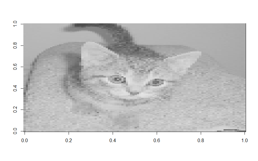
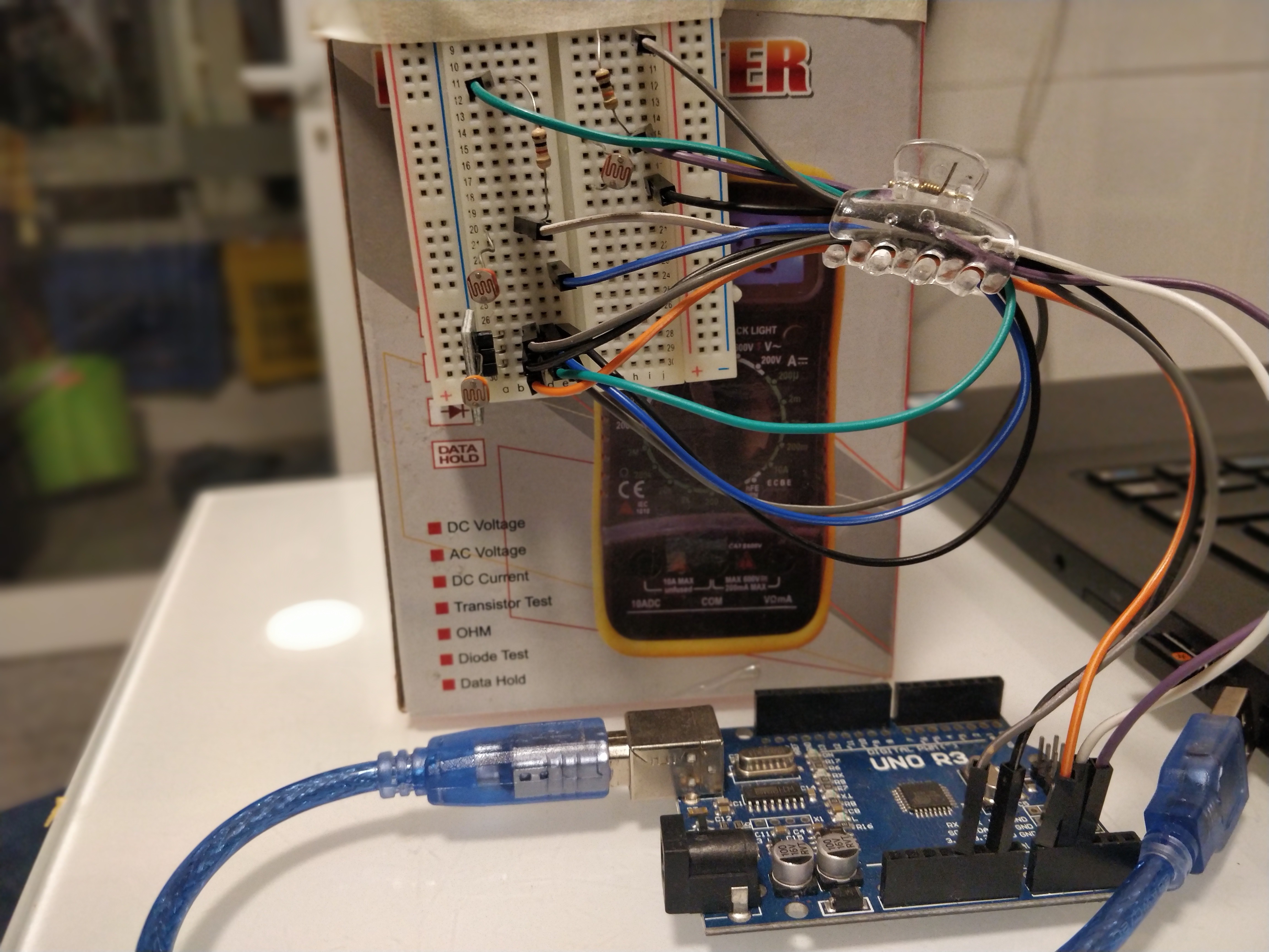
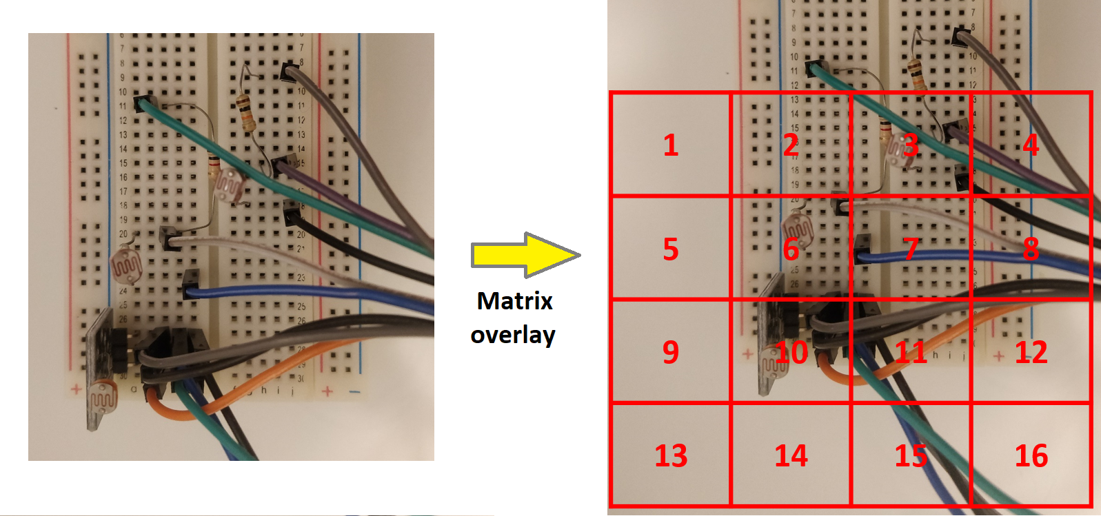
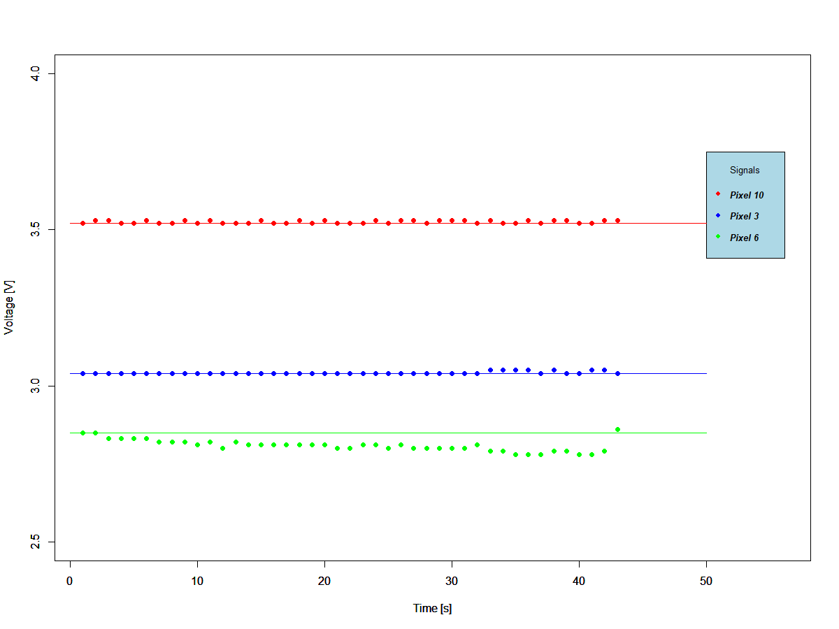
- Determine minimum requirements for sensor array
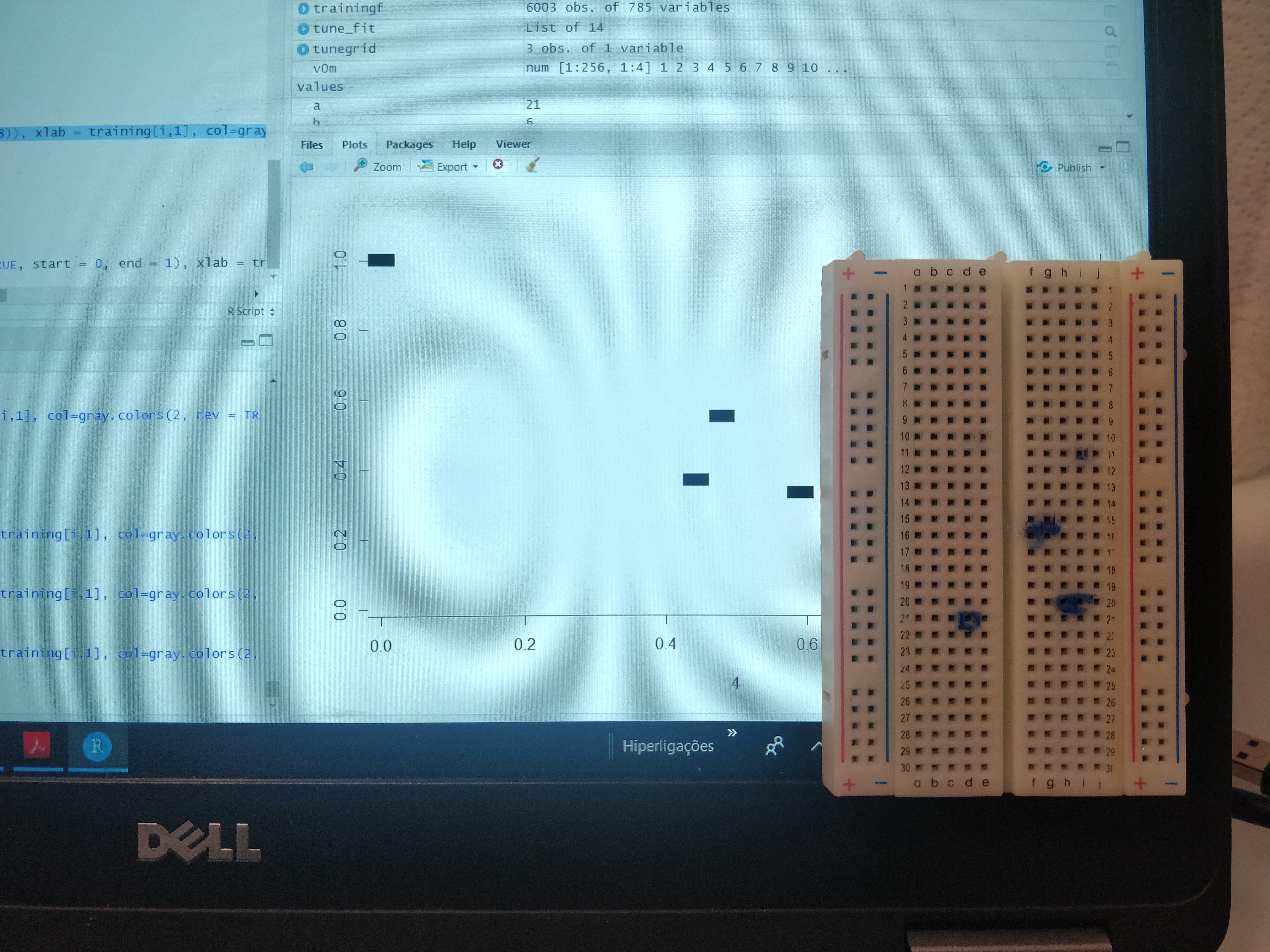
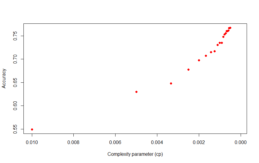
- Determine minimum requirements for ML model
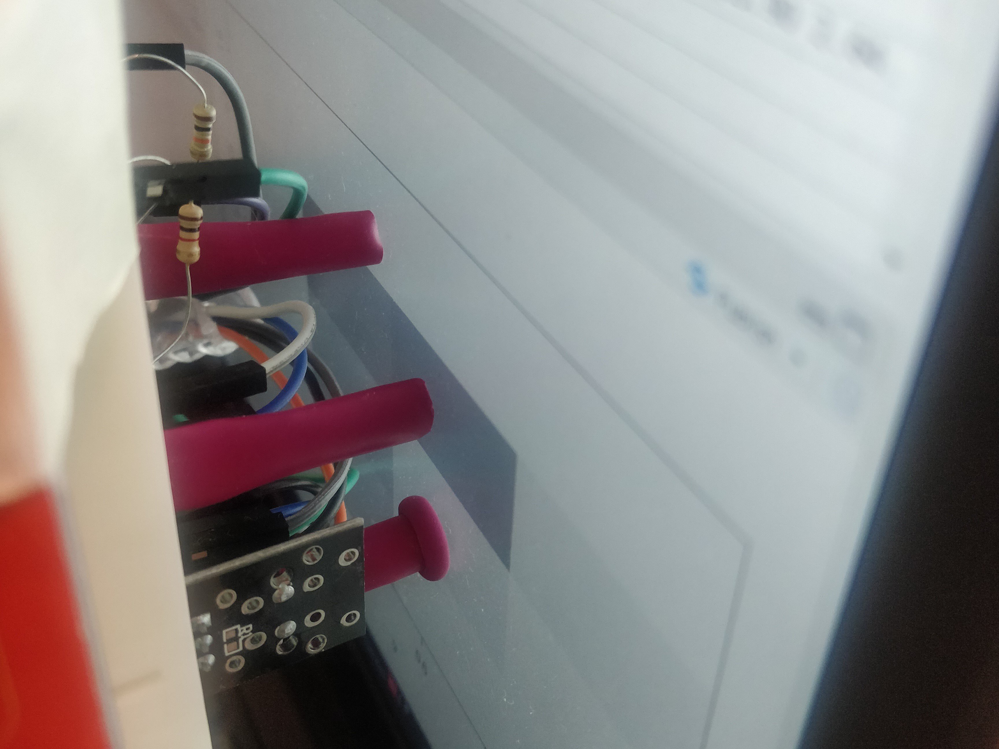
- Determine minimum requirements for object recognition hardware
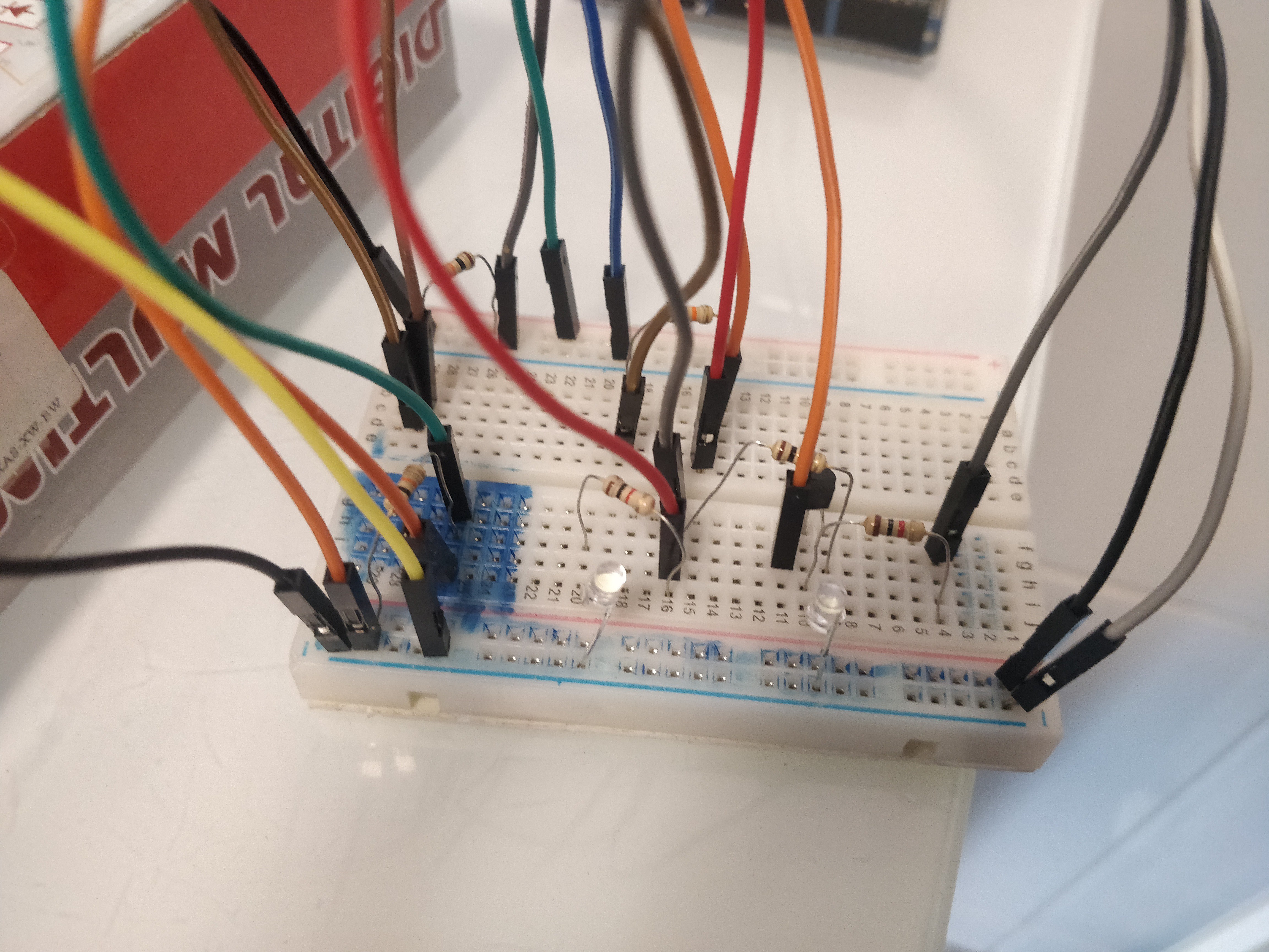
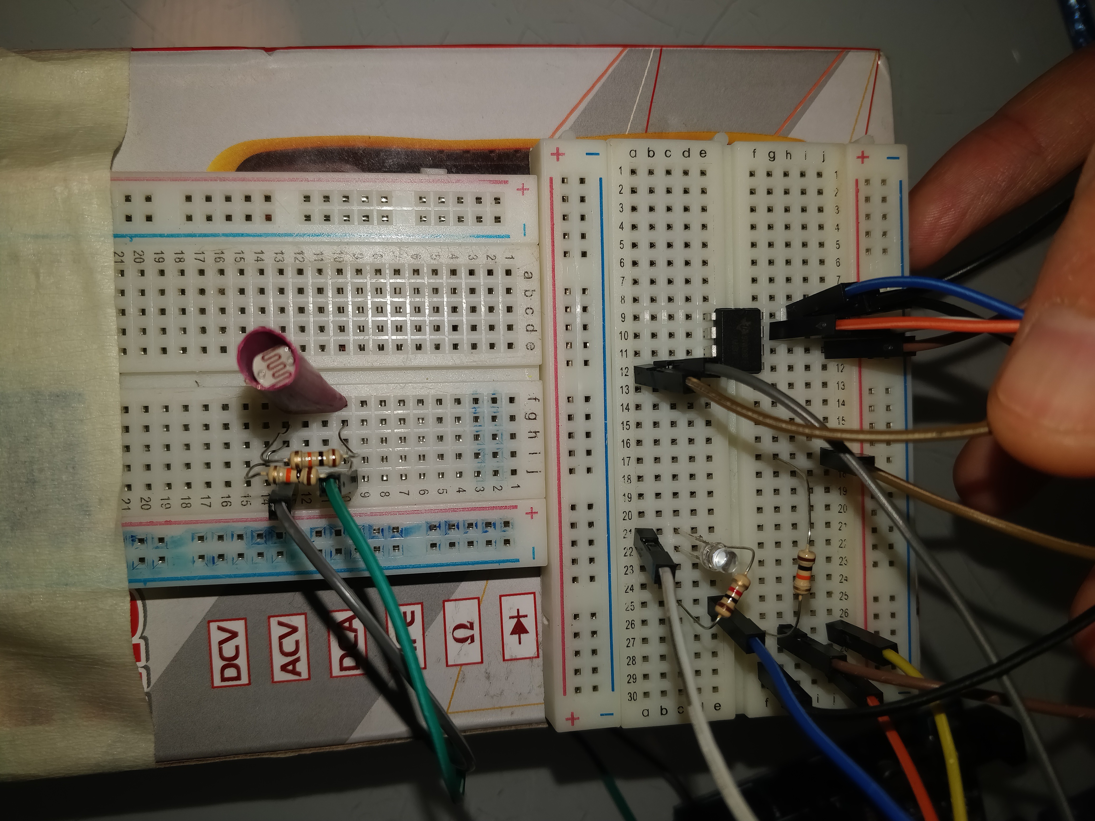
- Prototyping
- Final design
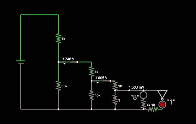
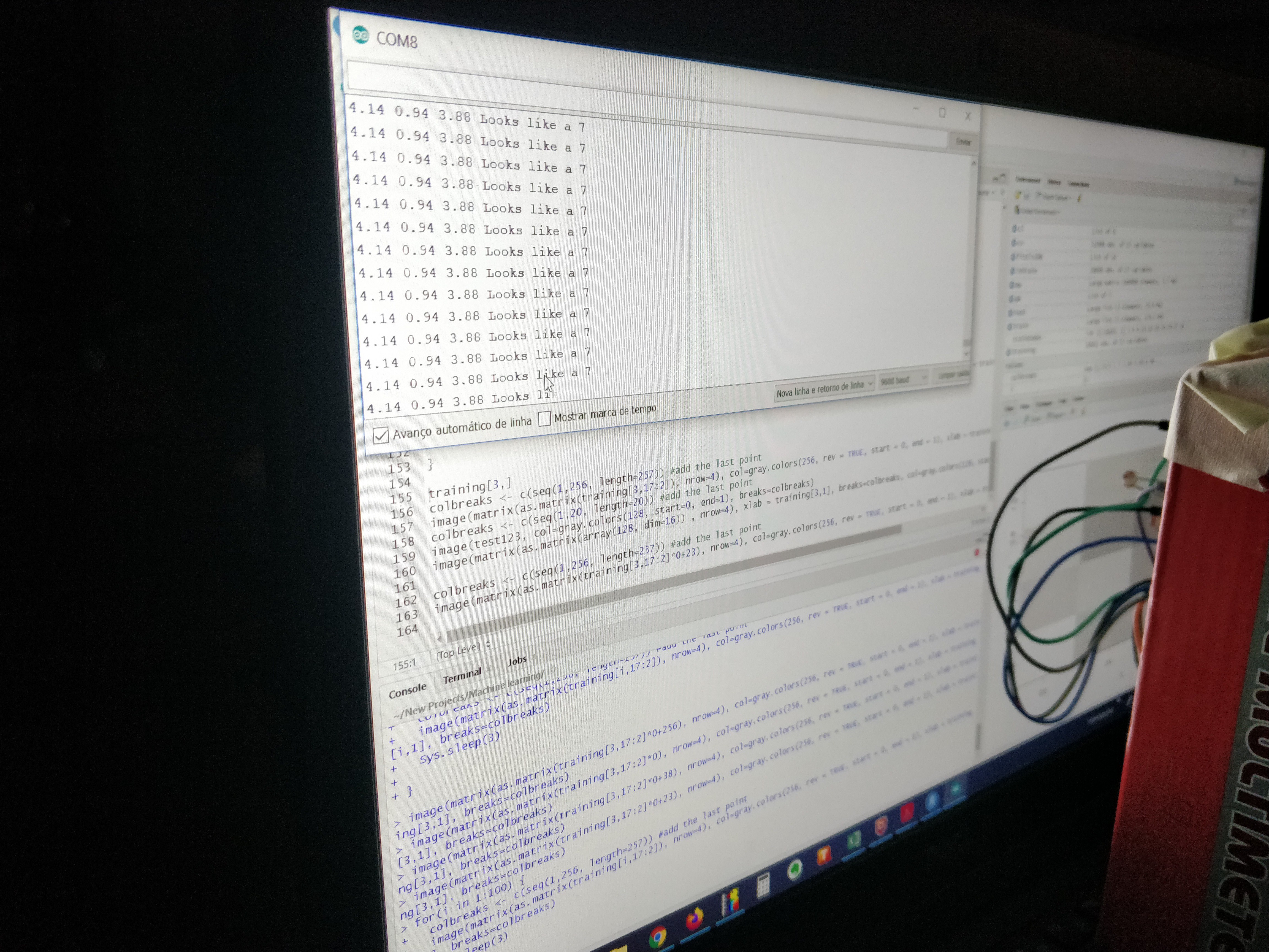
- Tests with a binary model signal
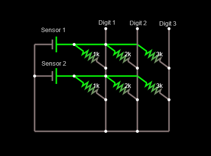
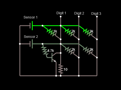
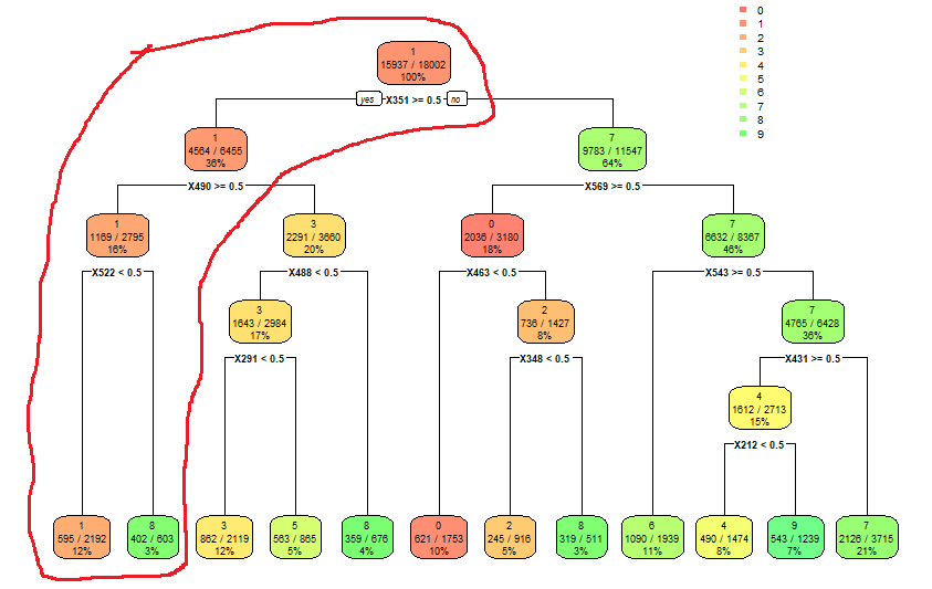
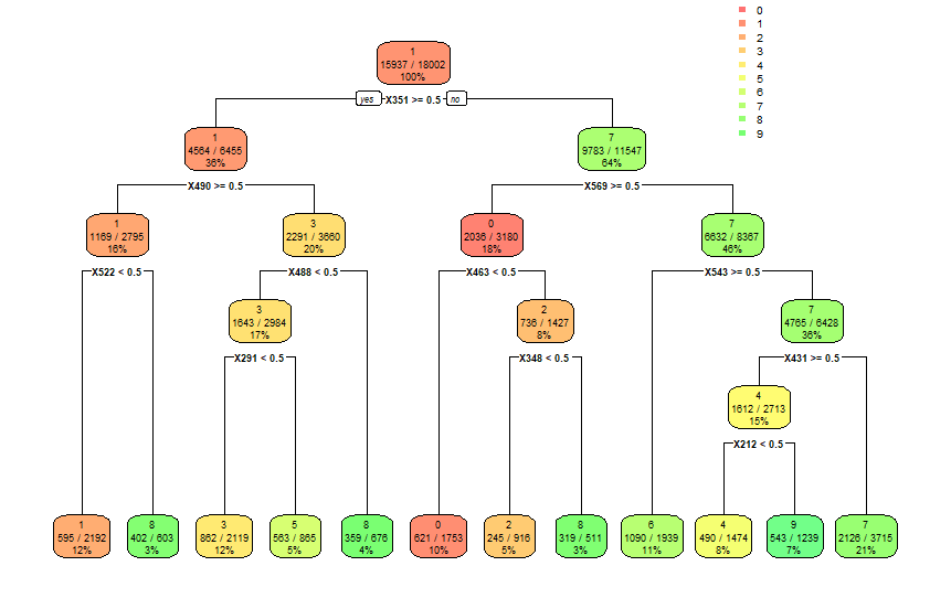
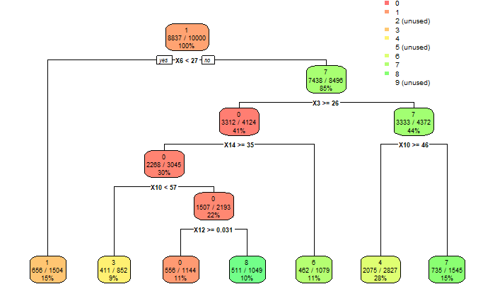
- Implementation of decision tree model using digital signal
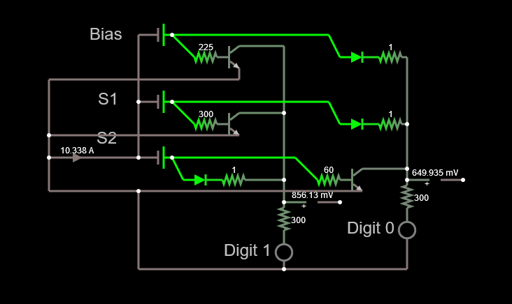
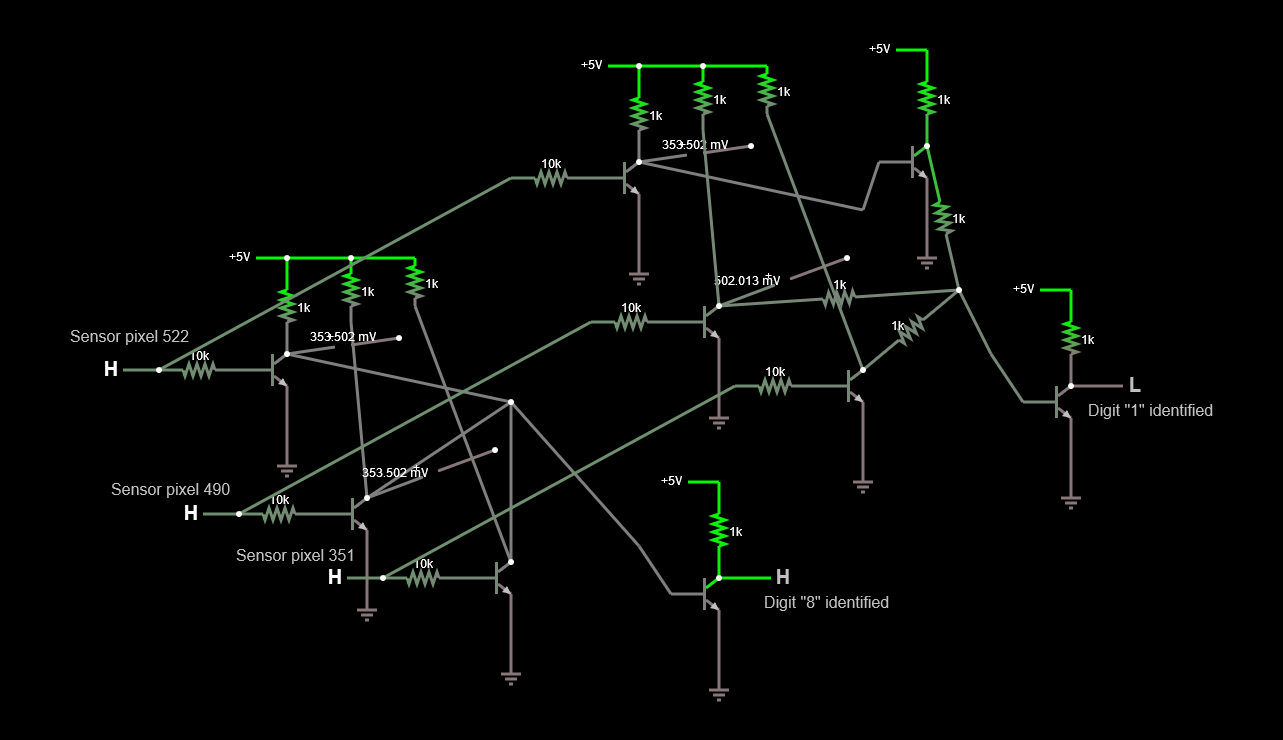
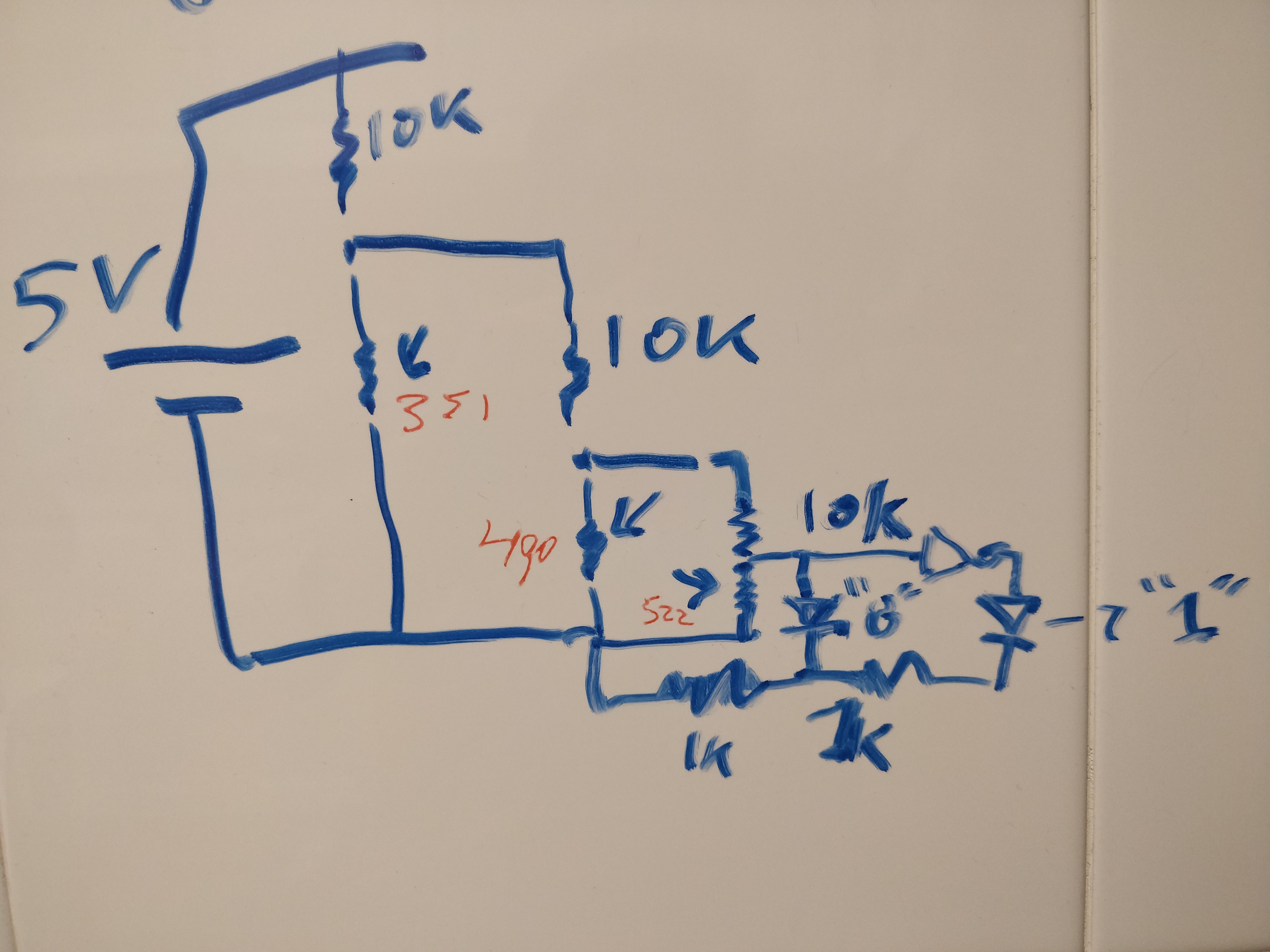
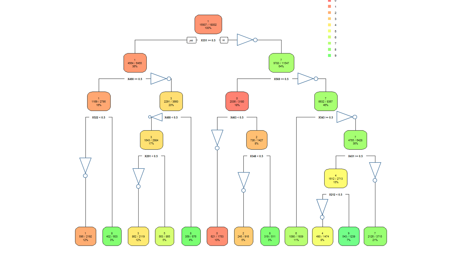
- Using resistor transistor logic for the Binary Decision tree
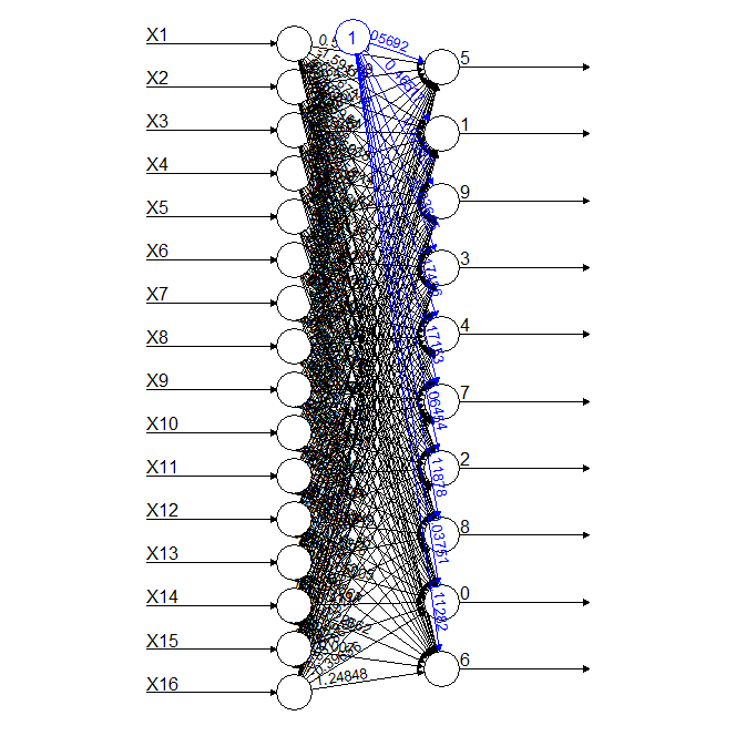
- Cats vs dogs, Random forests and Neural networks
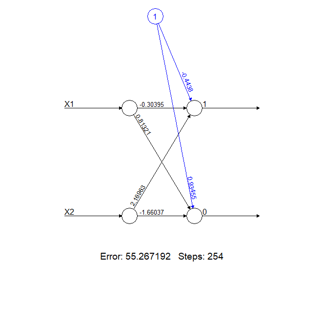
- Minimum model for discrete component neural networks
- Design of neural network nodes using discrete components
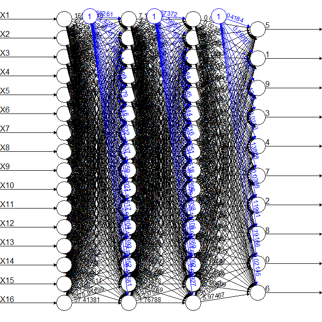
- PCB design of MNIST number recognition using discrete component neural network
- Translating a neural network to a discrete component memristor
The final objective is to have a system that is as close as possible to state of the art ML algorithms but implemented on discrete components for maximum speed at an acceptable complexity level.
Conclusion
The project was a partial success. Accuracy was below the objective of the project, nevertheless the concept worked for decision trees.
It has evolved in the meantime to include neural networks. Since where the project is going still fits the name it had on the day it started, it'll stay here for the time being.
The results showed significant potential for AI on discrete components, using sensors to obtain either analog or digital signals and allowing a tunable trade-off between complexity and accuracy.
 Of course a higher pixel density will improve the accuracy of the model but I'm more interested for the time being in simplicity at the expense of accuracy.
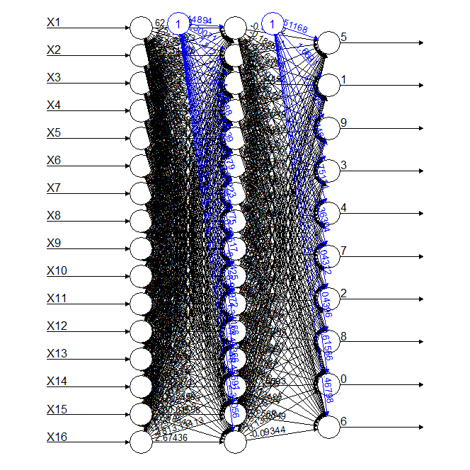


 Jithin
 int-smart
 jaromir.sukuba
 numero_trey
A couple of thoughts...
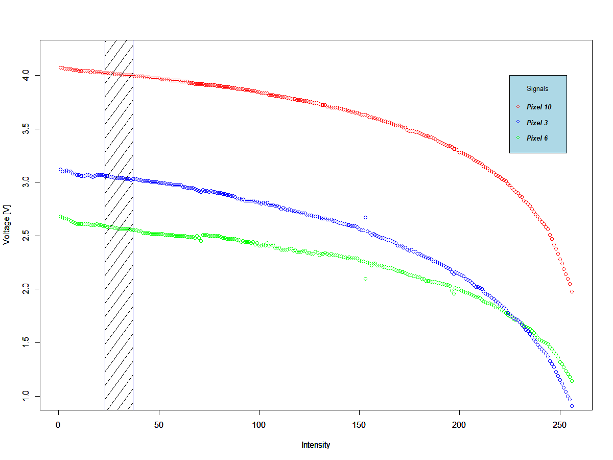
One, LDRs have *unbelievably* coarse tolerances. You are absolutely guaranteed to have to calibrate your voltage dividers individually, to even out all the imbalances they cause. A better choice might be an array of BPW34 photodiodes each driving JFETs -- photodiodes are photovoltaic devices (in fact, your standard solar cell is just a really massive photodiode) instead of being photoresistive. Yes, it increases overall component count, but repeatability and scalability to larger production and application numbers/cases goes up almost infinitely because you don't have to spend multiple afternoons arguing with the sensors to get it to work in the first place.
Two, back in the days of 8bit CPUs being common, and when microcontrollers were still "one-chip microcomputers" because the term "microcontroller" had yet to really catch on, NatSemi put out a bunch of ADC#### chips (that's "ADC" followed by a four-digit number -- ignore the rest of the name, it's almost always just packaging info) that were really good stuff. You can still get a bunch of em on eBay if you look for em right. "NOS" ("New Old Stock" -- i.e., purchased several years in the distant past and then promptly shoved in a drawer, never to be retrieved or used, until recently pulled out for sale) is the keyword there.
Three, if all else fails -- https://en.wikipedia.org/wiki/Resistor_ladder ;)